Strategies
Introduction
Pine Script® Strategies are specialized scripts that simulate trades across historical and realtime bars, allowing users to backtest and forward test their trading systems. Strategy scripts have many of the same capabilities as indicator scripts, and they provide the ability to place, modify, and cancel hypothetical orders and analyze performance results.
When a script uses the strategy() function as its declaration statement, it gains access to the strategy.* namespace, which features numerous functions and variables for simulating orders and retrieving essential strategy information. It also displays relevant information and simulated performance results in the dedicated Strategy Tester tab.
A simple strategy example
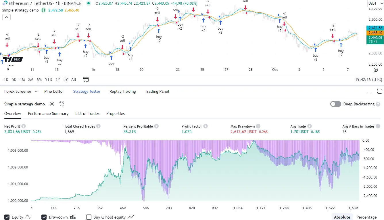
The following script is a simple strategy that simulates entering a long or short position when two moving averages cross. When the fastMA crosses above the slowMA, it places a “buy” market order to enter a long position. When the fastMA crosses below the slowMA, it places a “sell” market order to enter a short position:
Note that:
- The strategy() function call declares that the script is a strategy named “Simple strategy demo” that displays visuals on the main chart pane.
- The
margin_longandmargin_shortarguments in the strategy() call specify that the strategy must have 100% of a long or short trade’s amount available to allow the trade. See this section for more information. - The strategy.entry() function is the command that the script uses to create entry orders and reverse positions. The “buy” entry order closes any short position and opens a new long position. The “sell” entry order closes any long position and opens a new short position.
Applying a strategy to a chart
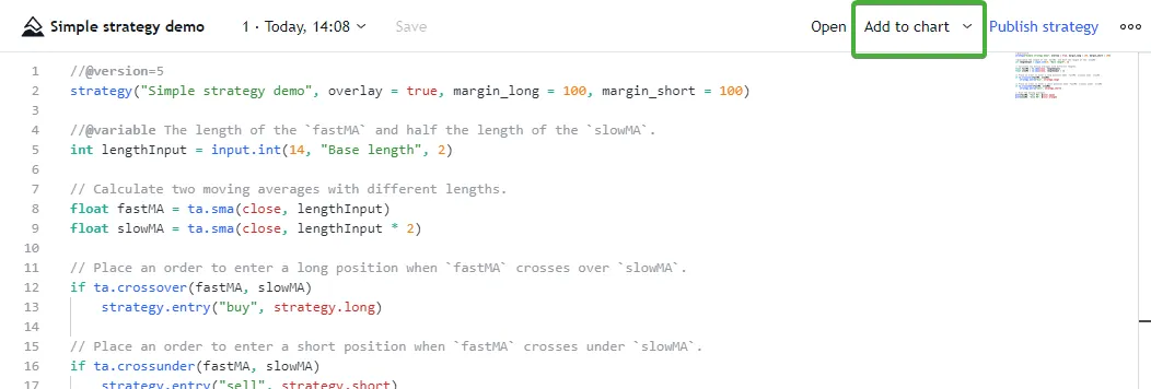
To test a strategy, add it to the chart. Select a built-in or published strategy from the “Indicators, Metrics & Strategies” menu, or write a custom strategy in the Pine Editor and click the “Add to chart” option in the top-right corner:
The script plots trade markers on the main chart pane and displays simulated performance results inside the Strategy Tester tab:
Strategy Tester
The Strategy Tester visualizes the hypothetical performance of a strategy script and displays its properties. To use it, add a script declared with the strategy() function to the chart, then open the “Strategy Tester” tab. If two or more strategies are on the chart, specify which one to analyze by selecting its name in the top-left corner.
After the selected script executes across the chart’s data, the Strategy Tester populates the following four tabs with relevant strategy information:
Overview
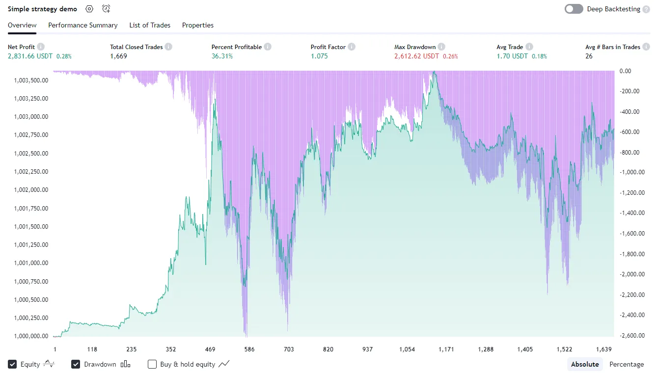
The Overview tab provides a quick look into a strategy’s performance over a sequence of simulated trades. This tab displays essential performance metrics and a chart with three helpful plots:
- The Equity baseline plot visualizes the strategy’s simulated equity across closed trades.
- The Drawdown column plot shows how far the strategy’s equity fell below its peak across trades.
- The Buy & hold equity plot shows the equity growth of a strategy that enters a single long position and holds that position throughout the testing range.
Note that:
- The chart has two separate vertical scales. The “Equity” and “Buy & hold equity” plots use the scale on the left, and the “Drawdown” plot uses the scale on the right. Users can toggle the plots and choose between absolute or percentage scales using the options at the bottom.
- When a user clicks on a point in this chart, the main chart scrolls to the corresponding bar where the trade closed and displays a tooltip containing the closing time.
Performance Summary
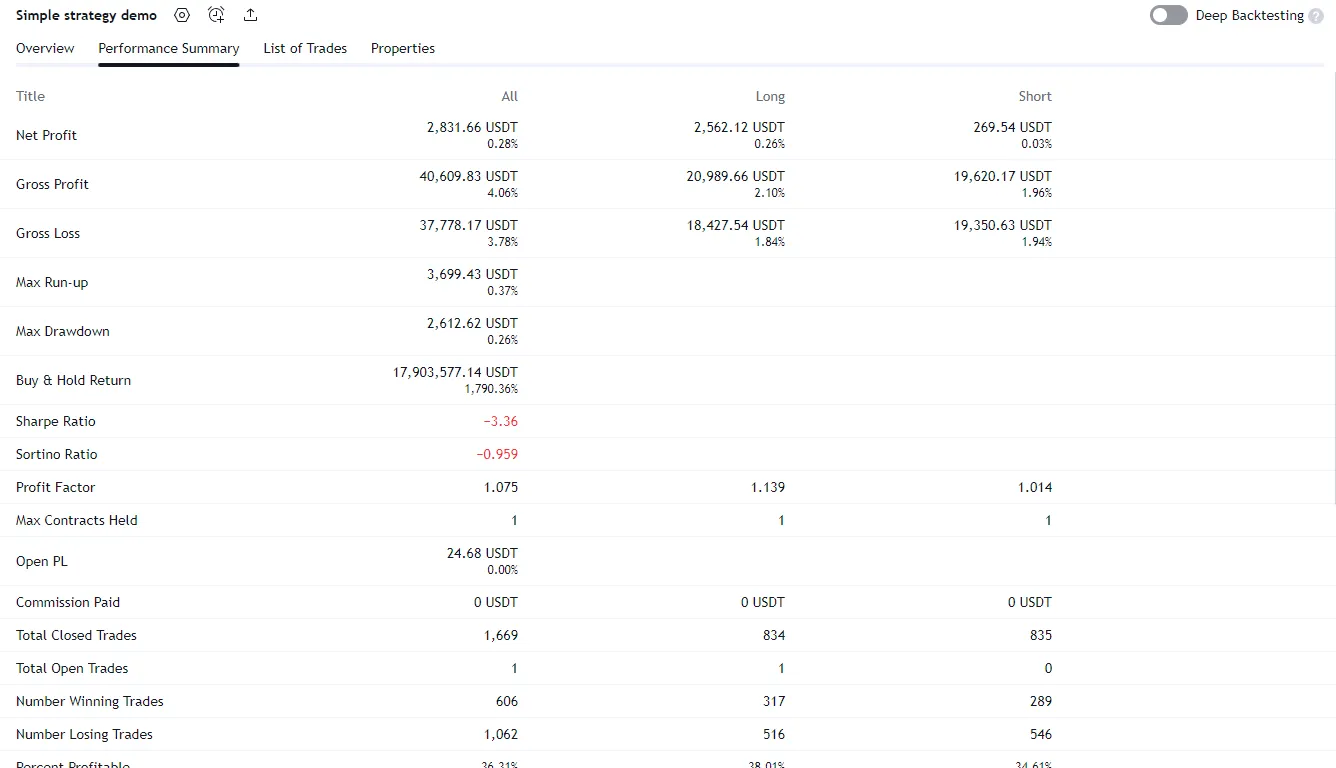
The Performance Summary tab presents an in-depth summary of a strategy’s key performance metrics, organized into separate columns. The “All” column shows performance information for all simulated trades, and the “Long” and “Short” columns show relevant metrics separately for long and short trades. This view provides more detailed insights into a strategy’s overall and directional trading performance:
List of Trades
The List of Trades tab chronologically lists a strategy’s simulated trades. Each item in the list displays vital information about a trade, including the dates and times of entry and exit orders, the names of the orders, the order prices, and the number of contracts/shares/lots/units. In addition, each item shows the trade’s profit or loss and the strategy’s cumulative profit, run-up, and drawdown:
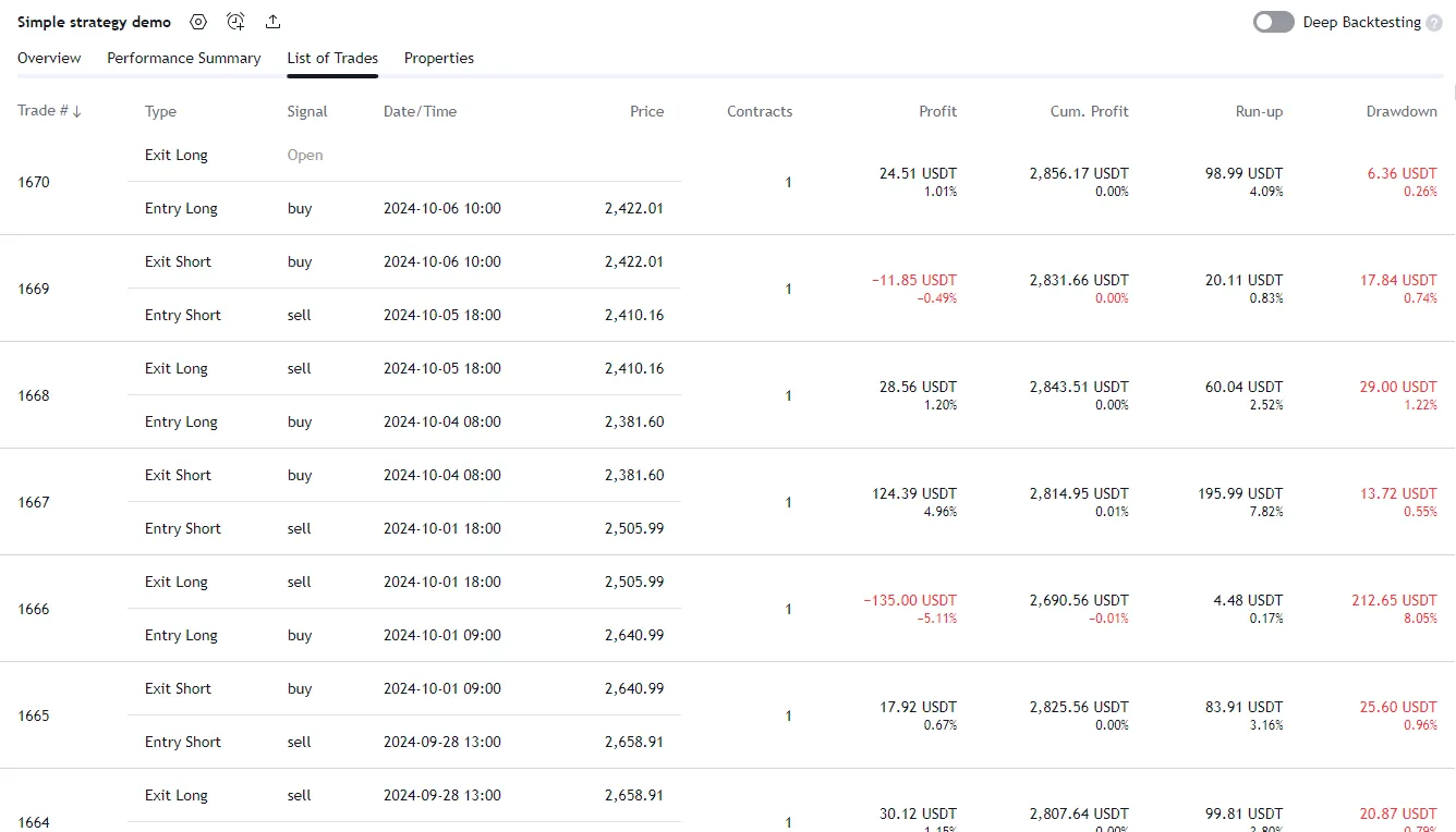
Note that:
- Hovering the mouse over a list item’s entry or exit information reveals a “Scroll to bar” button. Clicking that button navigates the main chart to the bar where the entry or exit occurred.
- The list shows each trade in descending order by default, with the latest trade at the top. Users can reverse this order by clicking the “Trade #” button above the list.
Properties
The “Properties” tab provides detailed information about a strategy’s configuration and the dataset that it executes across, organized into four collapsible sections:
- The “Date Range” section shows the range of dates that had simulated trades, and the overall available backtesting range.
- The “Symbol Info” section displays the chart’s symbol, timeframe, type, point value, currency, and tick size. It also includes the chart’s specified precision setting.
- The “Strategy Inputs” section lists the names and values of all the inputs available in the strategy’s “Settings/Inputs” tab. This section only appears if the script includes
input*()calls or specifies a nonzerocalc_bars_countargument in the strategy() declaration statement. - The “Strategy Properties” section provides an overview of the strategy’s properties, including the initial capital, account currency, order size, margin, pyramiding, commission, slippage, and other settings.

Broker emulator
TradingView uses a broker emulator to simulate trades while running a strategy script. Unlike in real-world trading, the emulator fills a strategy’s orders exclusively using available chart data by default. Consequently, it executes orders on historical bars after a bar closes. Similarly, the earliest point that it can fill orders on realtime bars is after a new price tick. For more information about this behavior, see the Execution model page.
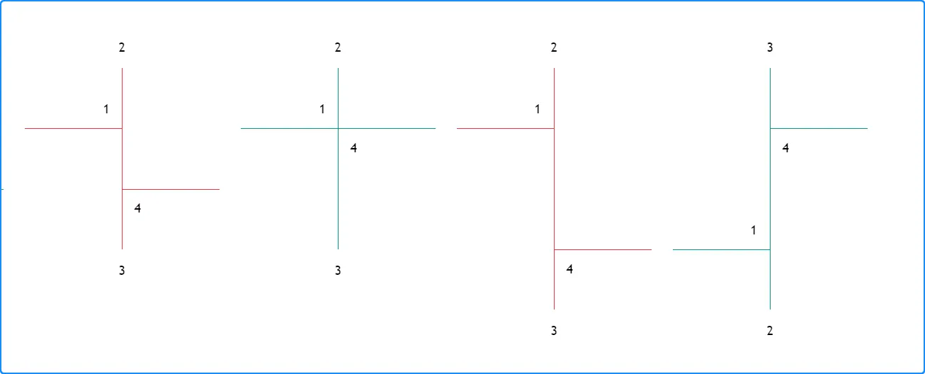
Because the broker emulator only uses price data from the chart by default, it makes assumptions about intrabar price movement when filling orders. The emulator analyzes the opening, high, low, and closing prices of chart bars to infer intrabar activity using the following logic:
- If the opening price of a bar is closer to the high than the low, the emulator assumes that the market price moved in this order: open → high → low → close.
- If the opening price of a bar is closer to the low than the high, the emulator assumes that the market price moved in this order: open → low → high → close.
- The emulator assumes no gaps exist between intrabars inside each chart bar, meaning it considers any value within a bar’s high-low range as a valid price for order execution.
- When filling price-based orders (all orders except market orders), the emulator assumes intrabars do not exist within the gap between the previous bar’s close and the current bar’s open. If the market price crosses an order’s price during the gap between two bars, the emulator fills the order at the current bar’s open and not at the specified price.
Bar magnifier
Users with Premium and higher-tier plans can override the broker emulator’s default assumptions about intrabar prices by enabling the Bar Magnifier backtesting mode. In this mode, the emulator uses data from lower timeframes to obtain more granular information about price action within bars, allowing more precise order fills in the strategy’s simulation.
To enable the Bar Magnifier mode, include use_bar_magnifier = true in the strategy() declaration statement, or select the “Using bar magnifier” option in the “Fill orders” section of the strategy’s “Settings/Properties” tab.
The following example script illustrates how the Bar Magnifier can enhance order-fill behavior. When the time of the bar’s open equals or exceeds the input time, it creates “Buy” and “Exit” limit orders at the calculated entryPrice and exitPrice. For visual reference, the script colors the background orange when it places the orders, and it draws two horizontal lines at the order prices. Here, we run the script on a weekly chart of “NASDAQ:MSFT
”:
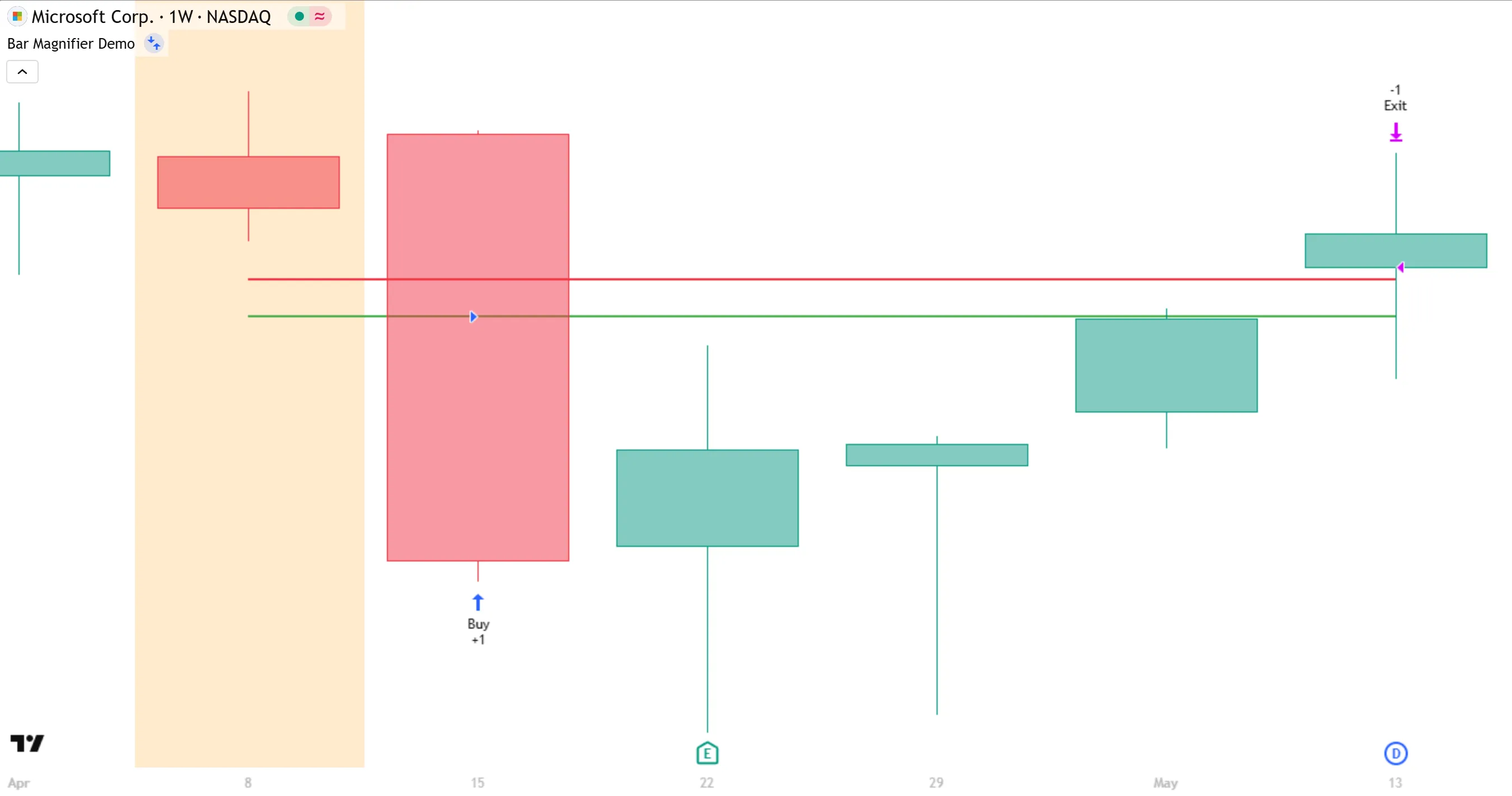
Because the script does not include use_bar_magnifier = true in its strategy() declaration, the broker emulator uses the default assumptions when filling the orders: that the bar’s price moved from open to high, high to low, and then low to close. Therefore, after filling the “Buy” order at the price indicated by the green line, the broker emulator inferred that the market price did not go back up to touch the red line and trigger the “Exit” order. In other words, the strategy could not enter and exit the position on the same bar, according to the broker emulator’s assumptions.
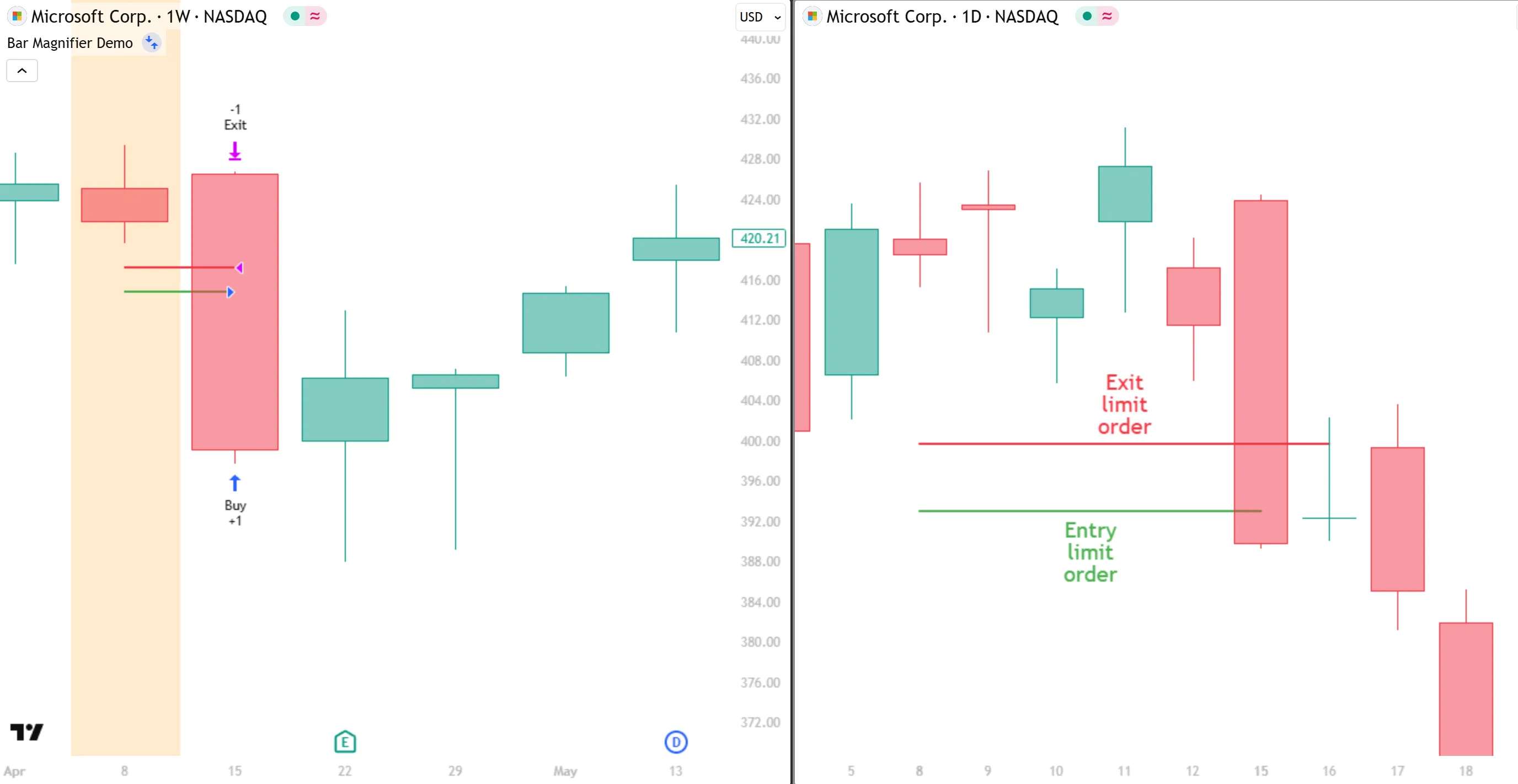
If we enable the Bar Magnifier mode, the broker emulator can access daily data on the weekly chart instead of relying on its assumptions about daily bars. On this timeframe, the market price did move back up to the “Exit” order’s price on the day after it reached the “Buy” order’s price. Below, we show the same weekly chart alongside the daily chart with the entry and exit lines annotated, to show the lower timeframe data that the Bar Magnifier used to execute both orders on the same bar:
Orders and trades
Pine Script strategies use orders to make trades and manage positions, similar to real-world trading. In this context, an order is an instruction that a strategy sends to the broker emulator to perform a market action, and a trade is the resulting transaction after the emulator fills an order.
Let’s take a closer look at how strategy orders work and how they become trades. Every 20 bars, the following script creates a long market order with strategy.entry() and draws a label. It calls strategy.close_all() on each bar from the global scope to generate a market order to close any open position:
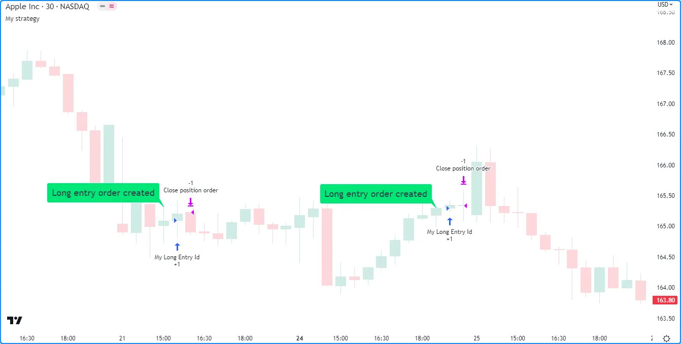
Note that:
- Although the script calls strategy.close_all() on every bar, the function only creates a new exit order when the strategy has an open position. If there is no open position, the function call has no effect.
The blue arrows on the above chart show where the strategy entered a long position, and the purple arrows mark the bars where the strategy closed the position. Notice that the label drawings appear one bar before the entry markers, and the entry markers appear one bar before the closing markers. This sequence illustrates order creation and execution in action.
By default, the earliest point the broker emulator fills an order is on the next available price tick, because creating and filling an order on the same tick is unrealistic. Since strategies recalculate after each bar closes by default, the next available tick where the emulator fills a generated order is at the open of the following bar. For example, when the longCondition occurs on bar 20, the script places an entry order to fill on the next tick, which is at the open of bar 21. When the strategy recalculates its values after bar 21 closes, it places an order to close the current position on the next tick, which is at the open of bar 22.
Order types
Pine Script strategies can simulate different order types to suit specific trading system needs. The main notable order types include market, limit, stop, and stop-limit.
Market orders
A market order is the simplest type of order, which most order placement commands generate by default. A market order is an instruction to buy or sell a security as soon as possible, irrespective of the price. As such, the broker emulator always executes a market order on the next available tick.
The example below alternates between placing a long and short market order once every lengthInput bars. When the bar_index is divisible by 2 * lengthInput, the strategy generates a long market order. Otherwise, it places a short market order when the bar_index is divisible by the lengthInput:
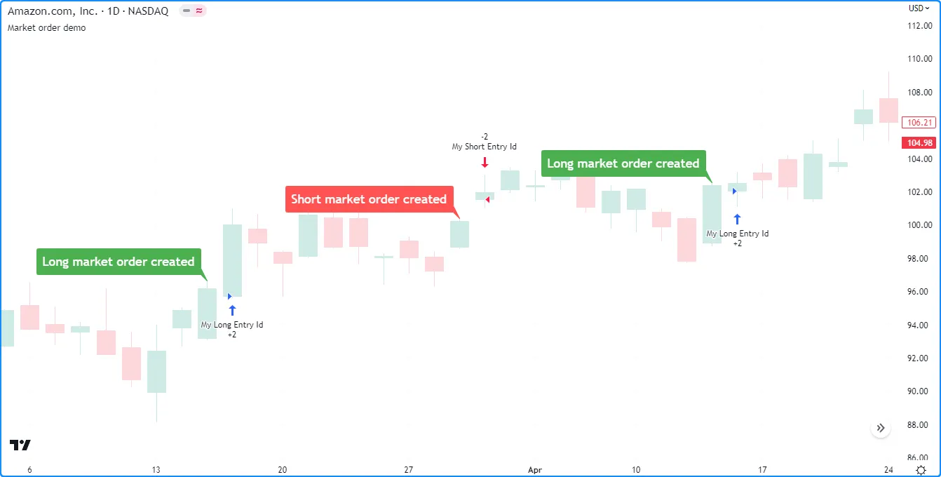
Note that:
- The labels indicate the bars where the script generates the market orders. The broker emulator fills each order at the open of the following bar.
- The strategy.entry() command can automatically reverse an open position in the opposite direction. See this section below for more information.
Limit orders
A limit order is an instruction to buy or sell a security at a specific price or better (lower than specified for long orders, and higher than specified for short orders), irrespective of the time. To simulate a limit order in a strategy script, pass a price value to the limit parameter of an applicable order placement command.
When the market price reaches a limit order’s value, or crosses it in the favorable direction, the broker emulator fills the order at that value or a better price. When a strategy generates a limit order at a worse value than the current market price (higher for long orders and lower for short orders), the emulator fills the order without waiting for the market price to reach that value.
For example, the following script generates a long limit order 800 ticks below the close of the bar 100 bars before the last chart bar using the strategy.entry() command. It draws a label to signify the bar where the strategy created the order and a line to visualize the order’s price:
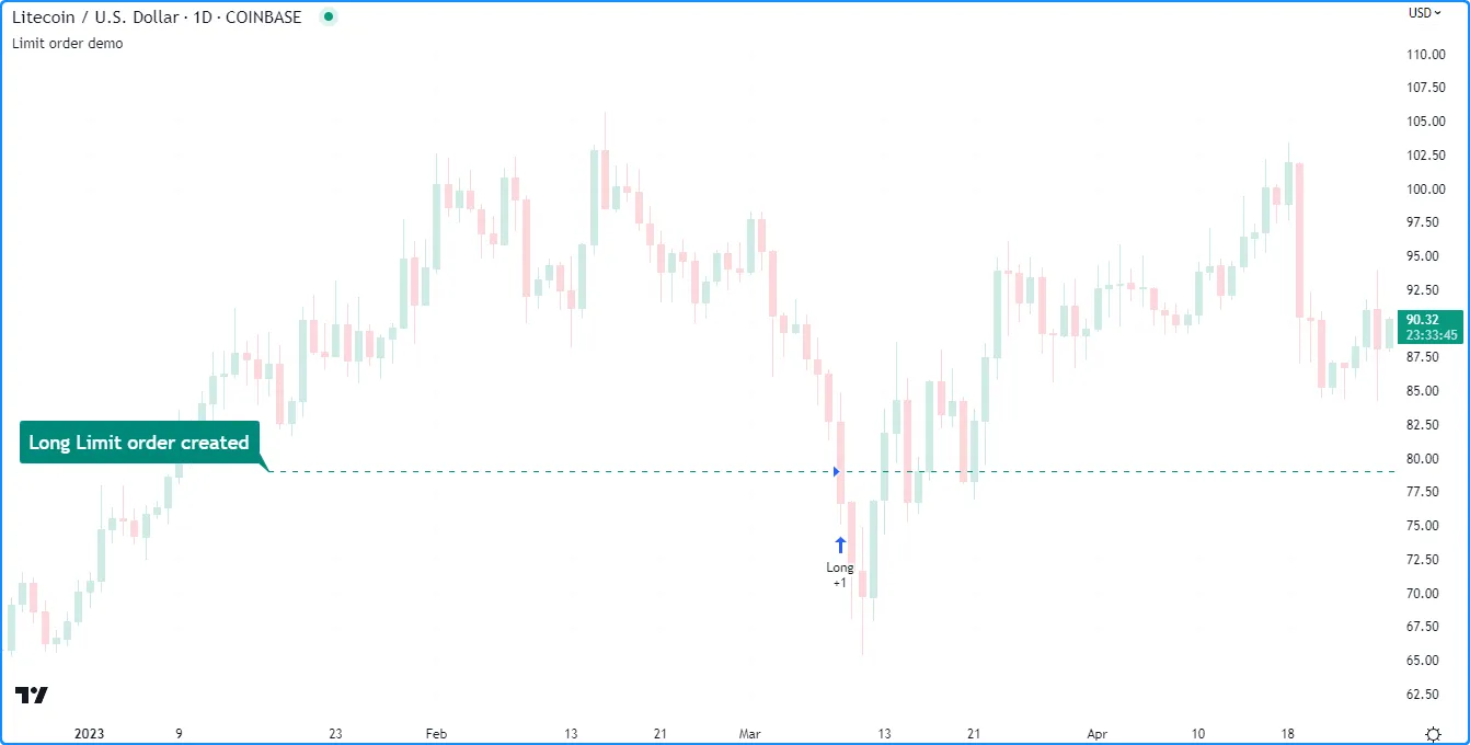
Notice that in the chart above, the label and the start of the line occurred several bars before the “Long” entry marker. The broker emulator could not fill the order while the market price remained above the limitPrice because such a price is a worse value for the long trade. After the price fell and reached the limitPrice, the emulator filled the order mid-bar at that value.
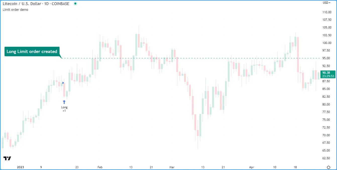
If we set the limitPrice to a value above the bar’s close rather than below, the broker emulator fills the order at the open of the following bar because the closing price is already a more favorable value for the long trade. Here, we set the limitPrice in the script to 800 ticks above the bar’s close to demonstrate this effect:
Stop and stop-limit orders
A stop order is an instruction to activate a new market or limit order when the market price reaches a specific price or a worse value (higher than specified for long orders and lower than specified for short orders). To simulate a stop order, pass a price value to the stop parameter of an applicable order placement command.
When a strategy generates a stop order at a better value than the current market price, it activates the subsequent order without waiting for the market price to reach that value.
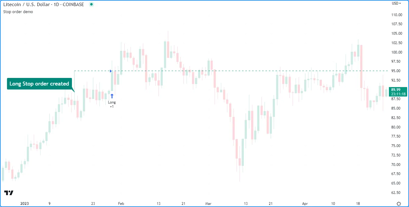
The following example calls strategy.entry() to place a stop order 800 ticks above the close 100 bars before the last historical chart bar. It also draws a label on the bar where it created the order and a line to display the stop price. As we see in the chart below, the strategy entered a long position immediately after the price crossed the stop level:
Note that:
- A basic stop order is essentially the opposite of a limit order in terms of its execution based on the market price. If we use a limit order instead of a stop order in this scenario, the order executes immediately on the next bar. See the previous section for an example.
When a strategy.entry() or strategy.order() call includes a stop and limit argument, it creates a stop-limit order. Unlike a basic stop order, which triggers a market order when the current price is at the stop level or a worse value, a stop-limit order creates a subsequent limit order to fill at the specified limit price.
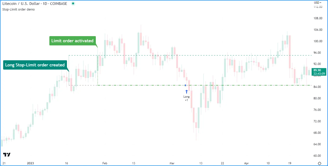
Below, we modified the previous script to simulate and visualize a stop-limit order. This script version includes the bar’s low as the limit price in the strategy.entry() command. It also includes additional drawings to show where the strategy activated the subsequent limit order and to visualize the limit price.
In this example chart, notice how the market price reached the limit level on the next bar after the stop-limit order was created, but the strategy did not enter a position because the limit order was not yet active. After price later reached the stop level, the strategy placed the limit order, and then the broker emulator filled it after the market price dropped back down to the limit level:
Order placement and cancellation
The strategy.* namespace features the following five functions that simulate the placement of orders, known as order placement commands: strategy.entry(), strategy.order(), strategy.exit(), strategy.close(), and strategy.close_all().
Additionally, the namespace includes the following two functions that cancel pending orders, known as order cancellation commands: strategy.cancel() and strategy.cancel_all().
The segments below explain these commands, their unique characteristics, and how to use them.
strategy.entry()
The strategy.entry() command generates entry orders. Its unique features help simplify opening and managing positions. This order placement command generates market orders by default. It can also create limit, stop, and stop-limit orders with the limit and stop parameters, as explained in the Order types section above.
Reversing positions
One of the strategy.entry() command’s unique features is its ability to reverse an open position automatically. By default, when an order from strategy.entry() executes while there is an open position in the opposite direction, the command automatically adds the position’s size to the new order’s size. The added quantity allows the order to close the current position and open a new position for the specified number of contracts/lots/shares/units in the new direction.
For instance, if a strategy has an open position of 15 shares in the strategy.long direction and calls strategy.entry() to place a new market order in the strategy.short direction, the size of the resulting transaction is the specified entry size plus 15 shares.
The example below demonstrates this behavior in action. When the buyCondition occurs once every 100 bars, the script calls strategy.entry() with qty = 15 to open a long position of 15 shares. Otherwise, when the sellCondition occurs on every 50th bar, the script calls strategy.entry() with qty = 5 to enter a new short position of five shares. The script also highlights the chart’s background on the bars where the buyCondition and sellCondition occurs:
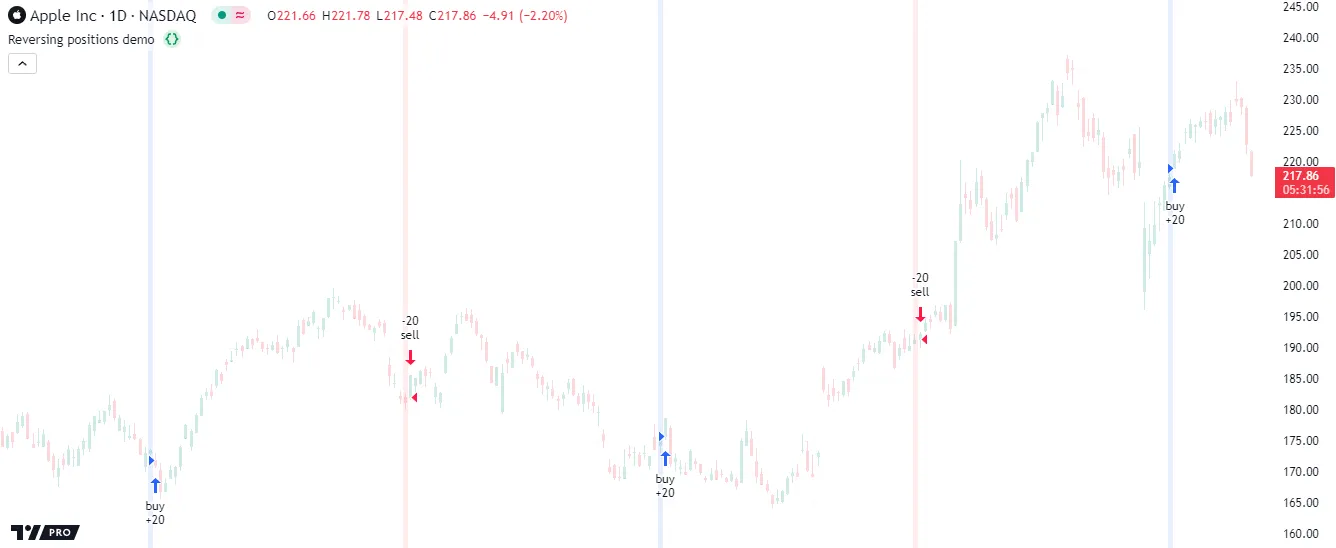
The trade markers on the chart show the transaction size, not the size of the resulting position. The markers above show that the transaction size was 20 shares on each order fill rather than 15 for long orders and five for short orders. Since strategy.entry() reverses a position in the opposite direction by default, each call adds the open position’s size (e.g., 15 for long entries) to the new order’s size (e.g., 5 for short entries), resulting in a quantity of 20 shares on each entry after the first. Although each of these transactions is 20 shares in size, the resulting positions are 5 shares for each short entry and 15 for each long entry.
Note that:
- The strategy.risk.allow_entry_in() function overrides the allowed direction for the strategy.entry() command. When a script specifies a trade direction with this risk management command, orders from strategy.entry() in the opposite direction close the open position without allowing a reversal.
Pyramiding
Another unique characteristic of the strategy.entry() command is its connection to a strategy’s pyramiding property. Pyramiding specifies the maximum number of successive entries a strategy allows in the same direction. Users can set this property by including a pyramiding argument in the strategy() declaration statement or by adjusting the “Pyramiding” input in the script’s “Settings/Properties” tab. The default value is 1, meaning the strategy can open new positions but cannot add to them using orders from strategy.entry() calls.
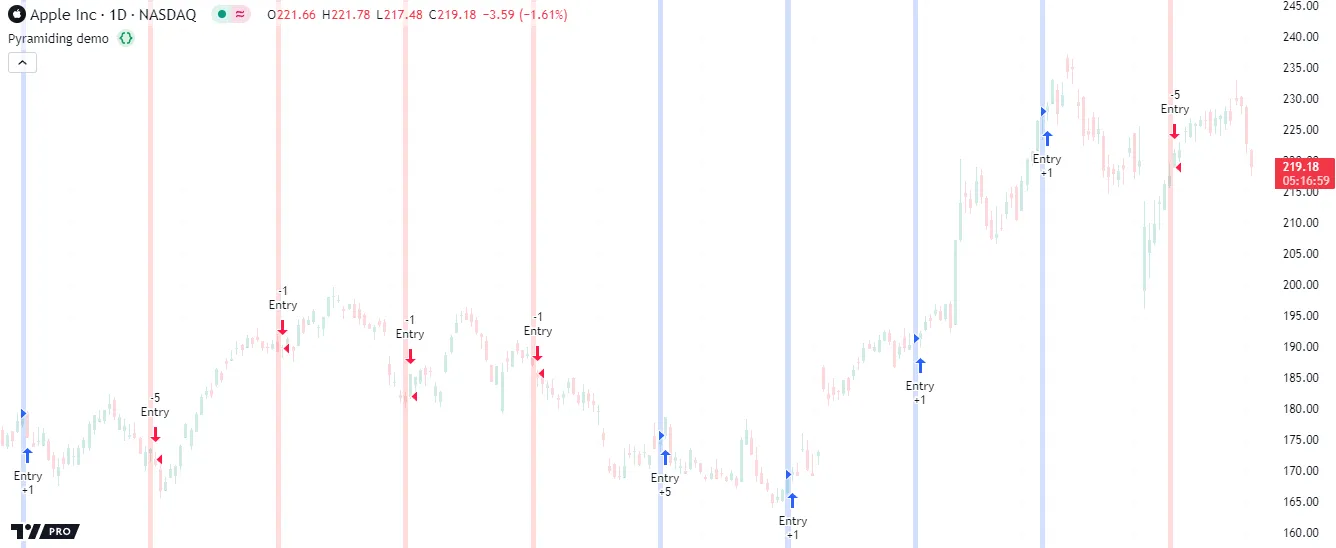
The following example uses strategy.entry() to place a market order when the entryCondition occurs on every 25th bar. The direction of the orders changes once every 100 bars, meaning every 100-bar cycle includes four strategy.entry() calls with the same direction. For visual reference of the conditions, the script highlights the chart’s background based on the current direction each time the entryCondition occurs:
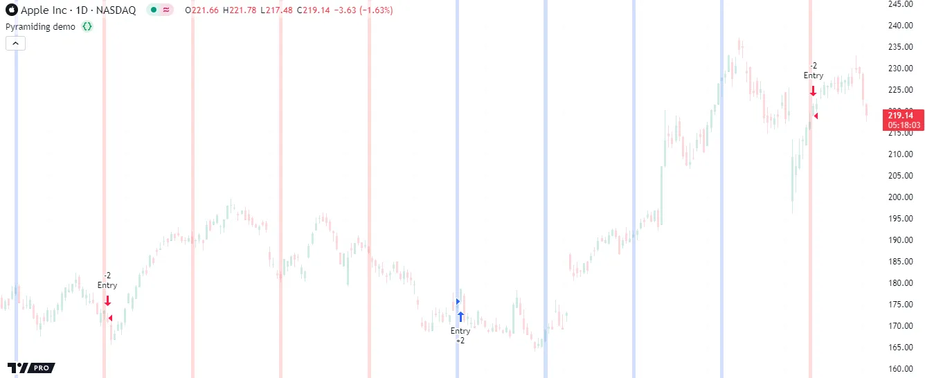
Notice that although the script calls strategy.entry() with the same direction four times within each 100-bar cycle, the strategy does not execute an order after every call. It cannot open more than one trade per position with strategy.entry() because it uses the default pyramiding value of 1.
Below, we modified the script by including pyramiding = 4 in the strategy() declaration statement to allow up to four successive trades in the same direction. Now, an order fill occurs after every strategy.entry() call:
strategy.order()
The strategy.order() command generates a basic order. Unlike other order placement commands, which can behave differently based on a strategy’s properties and open trades, this command ignores most properties, such as pyramiding, and simply creates orders with the specified parameters. This command generates market orders by default. It can also create limit, stop, and stop-limit orders with the limit and stop parameters. Orders from strategy.order() can open new positions and modify or close existing ones. When a strategy executes an order from this command, the resulting market position is the net sum of the open position and the filled order quantity.
The following script uses strategy.order() calls to enter and exit positions. The strategy places a long market order for 15 units once every 100 bars. On every 25th bar that is not a multiple of 100, it places a short market order for five units. The script highlights the background to signify where the strategy places a “buy” or “sell” order:
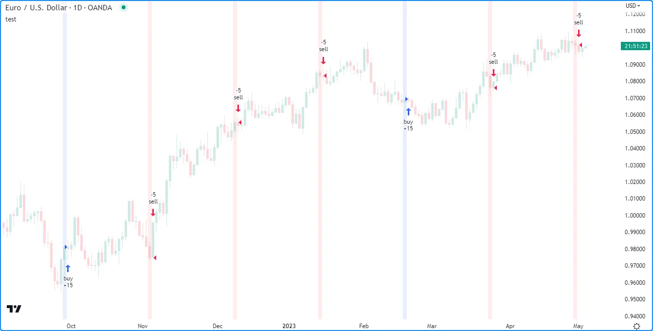
This particular strategy never simulates a short position. Unlike the strategy.entry() command, strategy.order() does not automatically reverse open positions. After filling a “buy” order, the strategy has an open long position of 15 units. The three subsequent “sell” orders reduce the position by five units each, and 15 - 5 * 3 = 0. In other words, the strategy opens a long position on every 100th bar and gradually reduces the size to 0 using three successive short orders. If we used strategy.entry() instead of the strategy.order() command in this example, the strategy would alternate between entering long and short positions of 15 and five units, respectively.
strategy.exit()
The strategy.exit() command generates exit orders. It features several unique behaviors that link to open trades, helping to simplify closing market positions and creating multi-level exits with take-profit, stop-loss, and trailing stop orders.
Unlike other order placement commands, which can generate a single order per call, each call to strategy.exit() can produce more than one type of exit order, depending on its arguments. Additionally, a single call to this command can generate exit orders for multiple entries, depending on the specified from_entry value and the strategy’s open trades.
Take-profit and stop-loss
The most basic use of the strategy.exit() command is the placement of limit orders to trigger exits after earning enough money (take-profit), stop orders to trigger exits after losing too much money (stop-loss), or both (bracket).
Four parameters determine the prices of the command’s take-profit and stop-loss orders:
- The
profitandlossparameters accept relative values representing the number of ticks the market price must move away from the entry price to trigger an exit. - The
limitandstopparameters accept absolute values representing the specific prices that trigger an exit when the market price reaches them.
When a strategy.exit() call includes arguments for the relative and absolute parameters defining take-profit or stop-loss levels (profit and limit or loss and stop), it creates orders only at the levels expected to trigger exits first.
For instance, if the profit distance is 19 ticks and the limit level is 20 ticks past the entry price in the favorable direction, the strategy.exit() command places a take-profit order profit ticks past the entry price because the market price will move that distance before reaching the limit value. In contrast, if the profit distance is 20 ticks and the limit level is 19 ticks past the entry price in the favorable direction, the command places a take-profit order at the limit level because the price will reach that value first.
The following example creates exit bracket (take-profit and stop-loss) orders with the strategy.exit() command. When the buyCondition occurs, the script calls strategy.entry() to place a “buy” market order. It also calls strategy.exit() with limit and stop arguments to create a take-profit order at the limitPrice and a stop-loss order at the stopPrice. The script plots the limitPrice and stopPrice values on the chart to visualize the exit order prices:
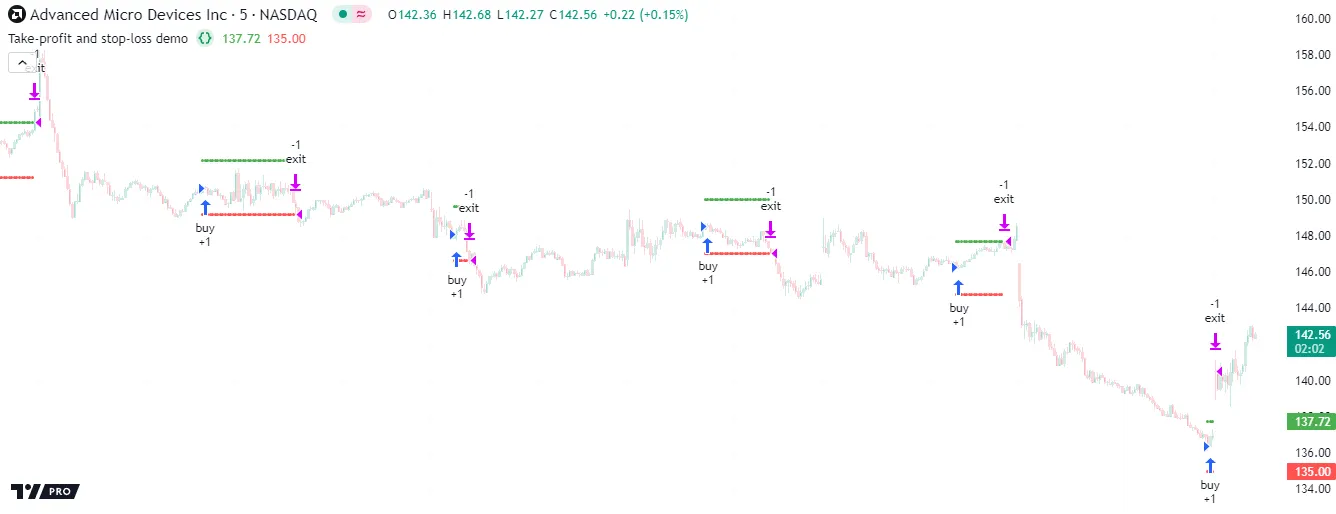
Note that:
- We did not specify a
qtyorqty_percentargument in the strategy.exit() call, meaning it creates orders to exit 100% of the “buy” order’s size. - The strategy.exit() command’s exit orders do not necessarily execute at the specified prices. Strategies can fill limit orders at better prices and stop orders at worse prices, depending on the range of values available to the broker emulator.
When a strategy.exit() call includes a from_entry argument, the resulting exit orders only apply to existing entry orders that have a matching ID. If the specified from_entry value does not match the ID of any entry in the current position, the command does not create any exit orders.
Below, we changed the from_entry argument of the strategy.exit() call in our previous script to “buy2”, which means it creates exit orders only for open trades with the “buy2” entry ID. This version does not place any exit orders because it does not create any entry orders with the “buy2” ID:
Note that:
- When a strategy.exit() call does not include a
from_entryargument, it creates exit orders for all the position’s open trades, regardless of their entry IDs. See the Exits for multiple entries section below to learn more.
Partial and multi-level exits
Strategies can use more than one call to strategy.exit() to create successive partial exit orders for the same entry ID, helping to simplify the formation of multi-level exit strategies. To use multiple strategy.exit() calls to exit from an open trade, include a qty or qty_percent argument in each call to specify how much of the traded quantity to close. If the sum of the exit order sizes exceeds the open position, the strategy automatically reduces their sizes to match the position.
Note that:
- When a strategy.exit() call includes both
qtyandqty_percentarguments, the command uses theqtyvalue to size the order and ignores theqty_percentvalue.
This example demonstrates a simple strategy that creates two partial exit order brackets for an entry ID. When the buyCondition occurs, the script places a “buy” market order for two shares with strategy.entry(), and it creates “exit1” and “exit2” brackets using two calls to strategy.exit(). The first call uses a qty of 1, and the second uses a qty of 3:
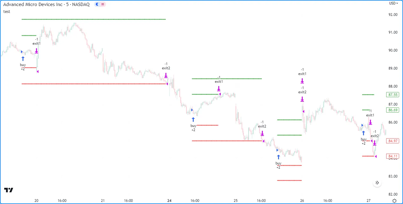
As we can see from the trade markers on the chart above, the strategy first executes the “exit1” take-profit or stop-loss order to reduce the open position by one share, leaving one remaining share in the position. However, we specified a size of three shares for the “exit2” order bracket, which exceeds the remaining position. Rather than using this specified quantity, the strategy automatically reduces the “exit2” orders to one share, allowing it to close the position successfully.
Note that:
- This strategy only fills one exit order from the “exit1” bracket, not both. When a strategy.exit() call generates more than one exit order type for an entry ID, the strategy fills the only the first triggered one and automatically cancels the others.
- The strategy reduced the “exit2” orders because all orders from the strategy.exit() calls automatically belong to the same strategy.oca.reduce group by default. Learn more about OCA groups below.
When creating multiple exit orders with different strategy.exit() calls, it’s crucial to note that the orders from each call reserve a portion of the open position. The orders from one strategy.exit() call cannot exit the portion of a position that a previous call already reserved.
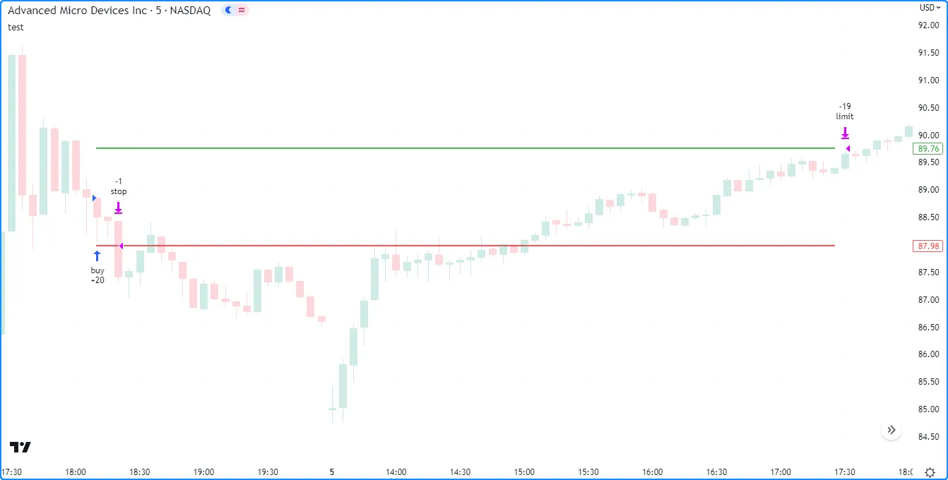
For example, this script generates a “buy” entry order for 20 shares with a strategy.entry() call and “limit” and “stop” exit orders with two separate calls to strategy.exit() 100 bars before the last chart bar. We specified a quantity of 19 shares for the “limit” order and 20 for the “stop” order:
Users unfamiliar with the strategy.exit() command’s unique behaviors might expect this strategy to close the entire market position if it fills the “stop” order before the “limit” order. However, the trade markers in the chart below show that the “stop” order only reduces the position by one share. The strategy.exit() call for the “limit” order executes first in the code, reserving 19 shares of the open position for closure with that order. This reservation leaves only one share available for the “stop” order to close, regardless of when the strategy fills it:
Trailing stops
One of the strategy.exit() command’s key features is its ability to create trailing stops, i.e., stop-loss orders that trail behind the market price by a specified amount whenever it moves to a better value in the favorable direction (upward for long positions and downward for short positions).
This type of exit order has two components: an activation level and a trail offset. The activation level is the value the market price must cross to activate the trailing stop calculation, and the trail offset is the distance the activated stop follows behind the price as it reaches successively better values.
Three strategy.exit() parameters determine the activation level and trail offset of a trailing stop order:
- The
trail_priceparameter accepts an absolute price value for the trailing stop’s activation level. - The
trail_pointsparameter is an alternative way to specify the activation level. Its value represents the tick distance from the entry price required to activate the trailing stop. - The
trail_offsetparameter accepts a value representing the order’s trail offset as a specified number of ticks.
To create and activate a trailing stop order, a strategy.exit() call must specify a trail_offset argument and either a trail_price or trail_points argument. If the call contains both trail_price and trail_points arguments, the command uses the level expected to activate the stop first. For instance, if the trail_points distance is 50 ticks and the trail_price value is 51 ticks past the entry price in the favorable direction, the strategy.exit() command uses the trail_points value to set the activation level because the market price will move that distance before reaching the trail_price level.
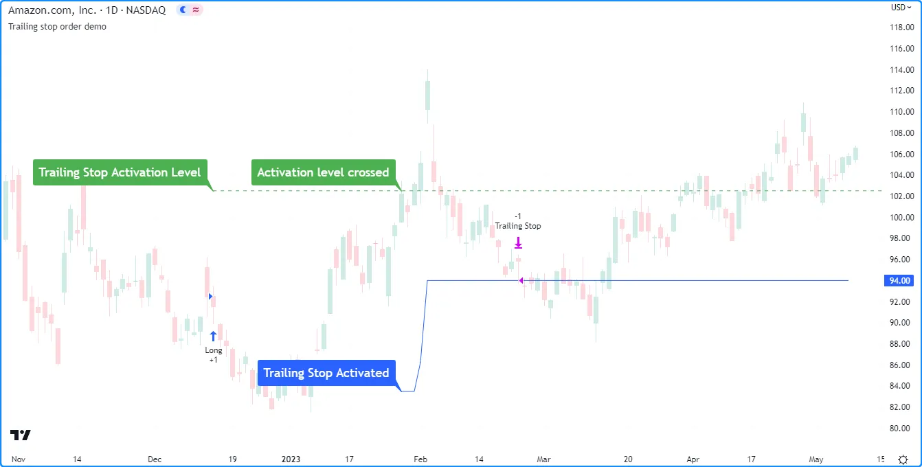
The example below demonstrates how a trailing stop order works in detail. The strategy places a “Long” market order with the strategy.entry() command 100 bars before the last chart bar, and it calls strategy.exit() with trail_price and trail_offset arguments on the following bar to create a trailing stop. The script uses lines, labels, and a plot to visualize the trailing stop’s behavior.
The green line on the chart shows the level the market price must reach to activate the trailing stop order. After the price reaches this level from below, the script uses a blue plot to display the trailing stop’s price. Each time the market price reaches a new high after activating the trailing stop, the stop’s price increases to maintain a distance of trailOffsetInput ticks from the best value. The exit order does not change its price level when the price decreases or does not reach a new high. Eventually, the market price crosses below the trailing stop, triggering an exit:
Exits for multiple entries
A single call to the strategy.exit() command can generate exit orders for more than one entry in an open position, depending on the call’s from_entry value.
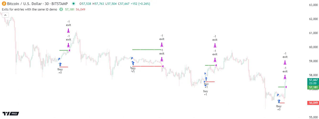
If an open position consists of two or more entries with the same ID, a single call to strategy.exit() with that ID as the from_entry argument places exit orders for each corresponding entry created before or on the bar where the call occurs.
For example, this script periodically calls strategy.entry() on two consecutive bars to enter and add to a long position. Both calls use “buy” as the id argument. After creating the second entry, the script calls strategy.exit() once with “buy” as its from_entry argument to generate separate exit orders for each entry with that ID. When the market price reaches the takeProfit or stopLoss value, the broker emulator fills two exit orders and closes the position:
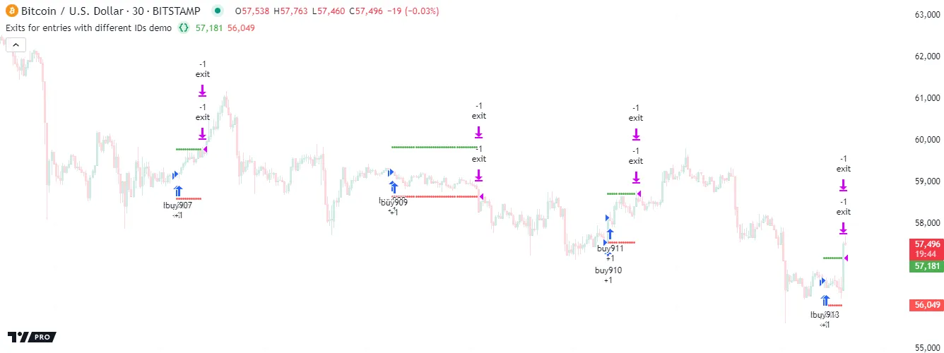
A single strategy.exit() call can also generate exit orders for all entries in an open position, irrespective of entry ID, when it does not include a from_entry argument.
Here, we changed the strategy.entry() instance in the above script to create an entry order with a distinct ID on each call, and we removed the from_entry argument from the strategy.exit() call. Since this version does not specify which entries the exit orders apply to, the strategy.exit() call creates orders for every entry in the position:
It’s crucial to note that a call to strategy.exit() without a from_entry argument persists and creates exit orders for all open trades in a position, regardless of when the entries occur. This behavior can affect strategies that manage positions with multiple entries or exits. When a strategy has an open position and calls strategy.exit() on any bar without specifying a from_entry ID, it generates exit orders for each entry created before or on that bar, and it continues to generate exit orders for subsequent entries after that bar until the position closes.
Let’s explore this behavior and how it works. The script below creates a long entry order with strategy.entry() on each bar within a user-specified time range, and it calls strategy.exit() without a from_entry argument on one bar within that range to generate exit orders for every entry in the open position. The exit command uses a loss value of 0, which means an exit order fills each time the market price is not above an entry order’s price.
The script prompts users to select three points before it starts its calculations. The first point specifies when order creation begins, the second determines when the single strategy.exit() call occurs, and the third specifies when order creation stops:
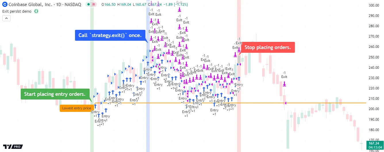
Note that:
- We included
pyramiding = 100in the strategy() declaration statement, which allows the position to have up to 100 open entries from strategy.entry(). - The script uses labels and bgcolor() to signify when order placement starts and stops and when the strategy.exit() call occurs.
- The script draws a line and a label at the lowest entry price to show the value the market price must reach to close the position.
We can observe the unique strategy.exit() behavior in this example by comparing the code itself with the script’s chart outputs. The script calls strategy.exit() one time, only on the bar with the blue label. However, this single call placed exit orders for every entry before or on that bar and continued placing exit orders for all entries after that bar. This behavior occurs because strategy.exit() has no way to determine when to stop placing orders if it does not link to entries with a specific ID. In this case, the command only ceases to create new exit orders after the position fully closes.
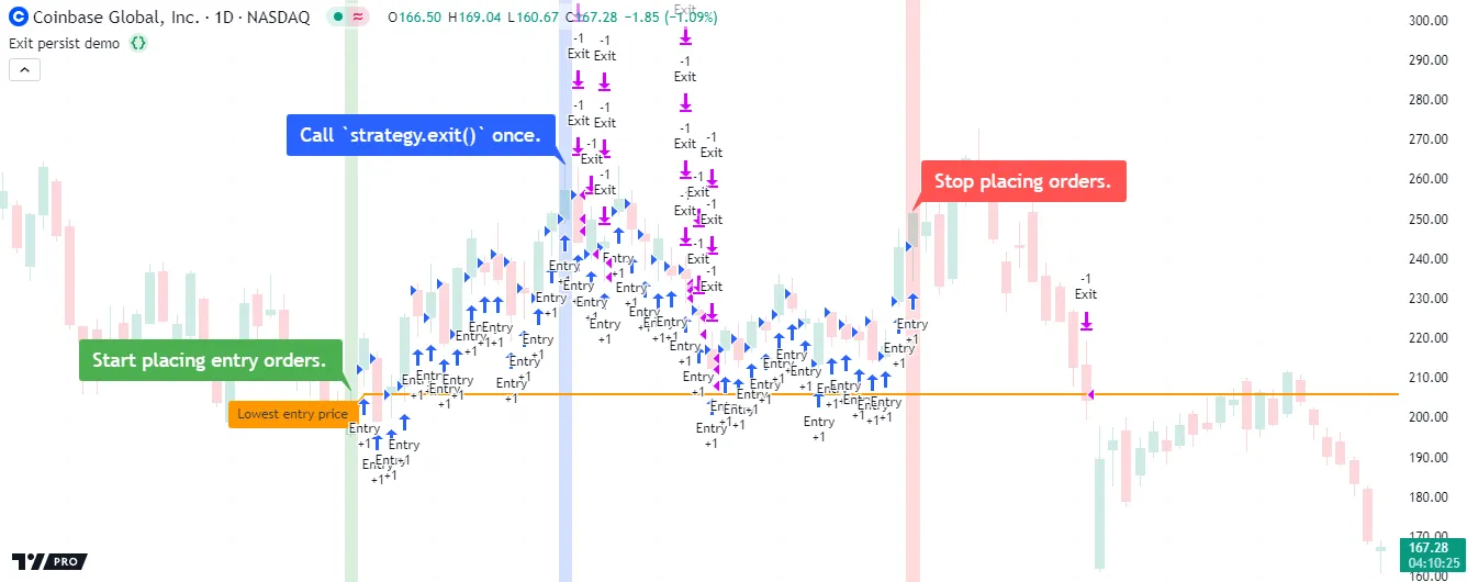
The above script would exhibit different behavior if we included a from_entry argument in the strategy.exit() call. When a call to this command specifies a from_entry ID, it only applies to entries with that ID which the strategy created before or on the bar of the call. The command does not place exit orders for subsequent entries created after that bar in that case, even ones with the same ID.
Here, we added from_entry = "Entry" to our script’s strategy.exit() call, meaning it only produces exit orders for entries with the “Entry” ID. Only 17 exits occur this time, each corresponding to an entry order created before or on the bar with the blue label. The call does not affect any entries that the strategy creates after that bar:
strategy.close() and strategy.close_all()
The strategy.close() and strategy.close_all() commands generate orders to exit from an open position. Unlike strategy.exit(), which creates price-based exit orders (e.g., stop-loss), these commands generate market orders that the broker emulator fills on the next available tick, irrespective of the price.
The example below demonstrates a simple strategy that places a “buy” entry order with strategy.entry() once every 50 bars and a market order to close the long position with strategy.close() 25 bars afterward:
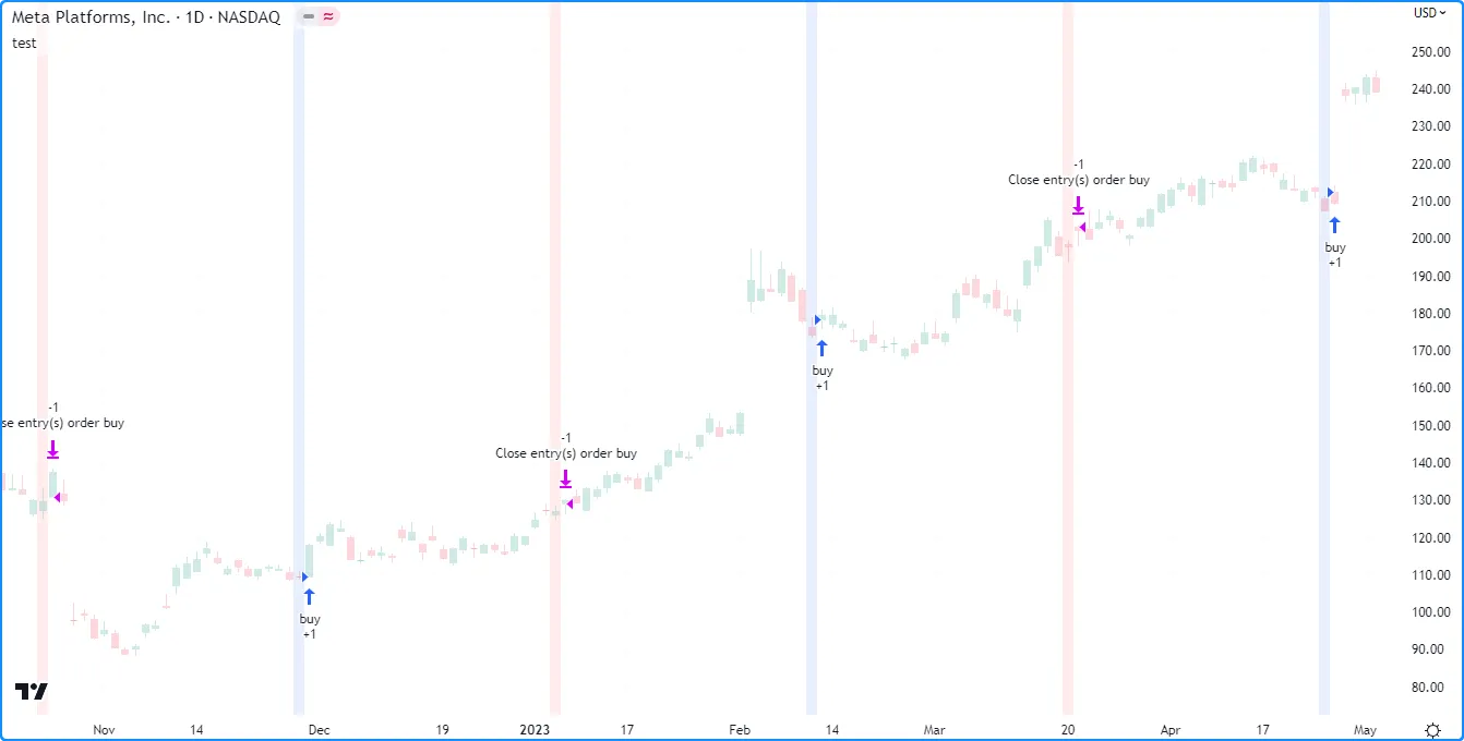
Notice that the strategy.close() call in this script uses “buy” as its required id argument. Unlike strategy.exit(), this command’s id parameter specifies the entry ID of an open trade. It does not represent the ID of the resulting exit order. If a market position consists of multiple open trades with the same entry ID, a single strategy.close() call with that ID as its id argument generates a single market order to exit from all of them.
The following script creates a “buy” order with strategy.entry() once every 25 bars, and it calls strategy.close() with “buy” as its id argument to close all open trades with that entry ID once every 100 bars. The market order from strategy.close() closes the entire position in this case because every open trade has the same “buy” entry ID:
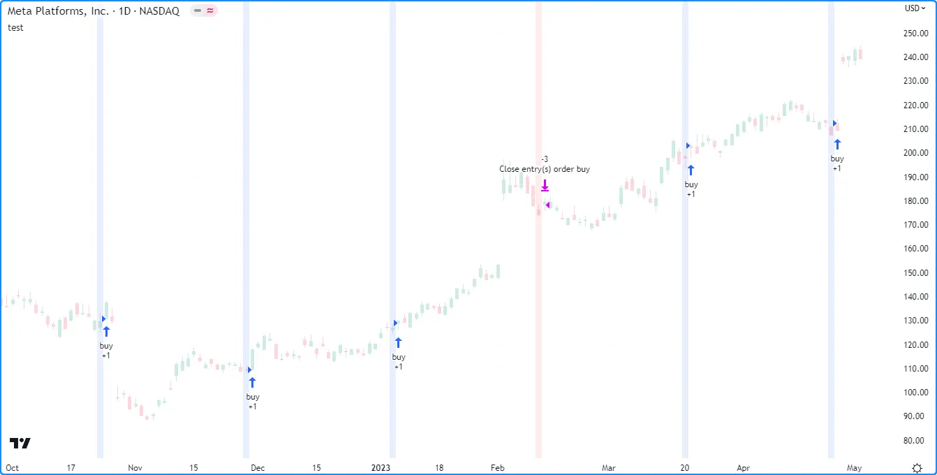
Note that:
- We included
pyramiding = 3in the strategy() declaration statement, allowing the script to generate up to three entries per position with strategy.entry() calls.
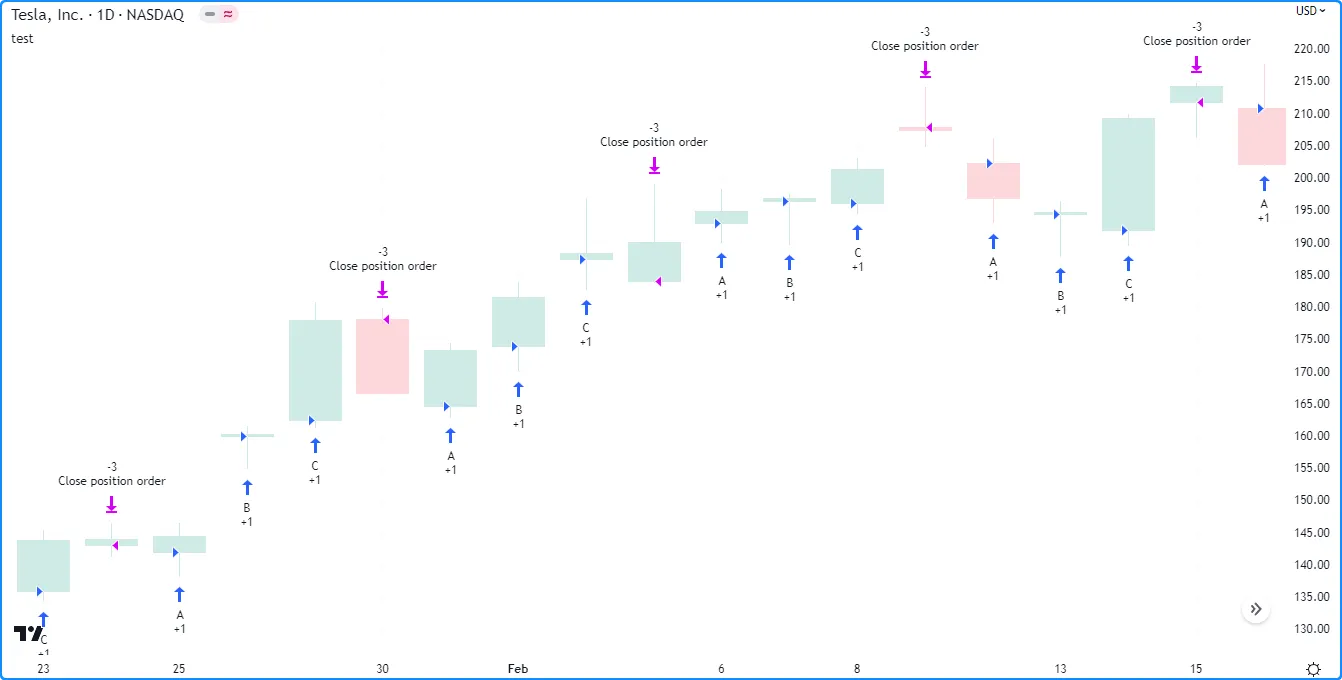
The strategy.close_all() command generates a market order to exit from the open position that does not link to any specific entry ID. This command is helpful when a strategy needs to exit as soon as possible from a position consisting of multiple open trades with different entry IDs.
The script below places “A”, “B”, and “C” entry orders sequentially based on the number of open trades as tracked by the strategy.opentrades variable, and then it calls strategy.close_all() to create a single order that closes the entire position on the following bar:
strategy.cancel() and strategy.cancel_all()
The strategy.cancel() and strategy.cancel_all() commands allow strategies to cancel unfilled orders before the broker emulator processes them. These order cancellation commands are most helpful when working with price-based orders, including all orders from strategy.exit() calls and the orders from strategy.entry() and strategy.order() calls that use limit or stop arguments.
The strategy.cancel() command has a required id parameter, which specifies the ID of the entry or exit orders to cancel. The strategy.cancel_all() command does not have such a parameter because it cancels all unfilled orders, regardless of ID.
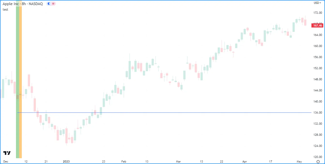
The following strategy places a “buy” limit order 500 ticks below the closing price 100 bars before the last chart bar with strategy.entry(), and it cancels the order on the next bar with strategy.cancel(). The script highlights the chart’s background to signify when it places and cancels the “buy” order, and it draws a horizontal line at the order’s price. As we see below, our example chart shows no entry marker when the market price crosses the horizontal line because the strategy already cancels the order (when the chart’s background is orange) before it reaches that level:
The strategy.cancel() command affects all unfilled orders with a specified ID. It does nothing if the specified id represents the ID of an order that does not exist. When there is more than one unfilled order with the specified ID, the command cancels all of them at once.
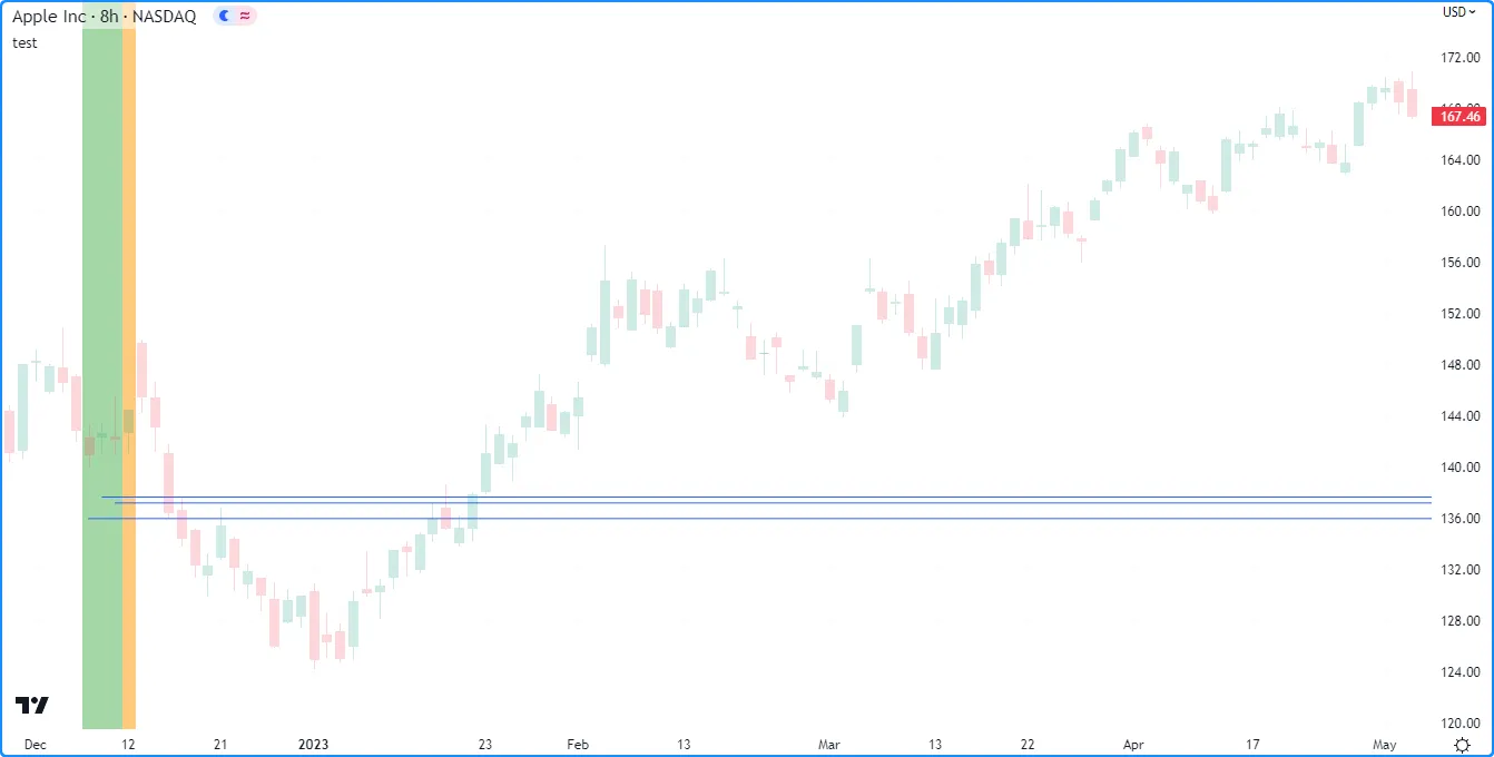
Below, we’ve modified the previous script to place a “buy” limit order on three consecutive bars, starting 100 bars before the last chart bar. After placing all three orders, the strategy cancels them using strategy.cancel() with “buy” as the id argument, resulting in nothing happening when the market price reaches any of the order prices (horizontal lines):
Note that:
- We included
pyramiding = 3in the strategy() declaration statement, allowing three successive entries from strategy.entry() per position. The script would also achieve the same result without this setting if it called strategy.order() instead because pyramiding does not affect orders from that command.
The strategy.cancel() and strategy.cancel_all() commands can cancel orders of any type, including market orders. However, it is important to note that either command can cancel a market order only if its call occurs on the same script execution as the order placement command. If the call happens after that point, it has no effect because the broker emulator fills market orders on the next available tick.
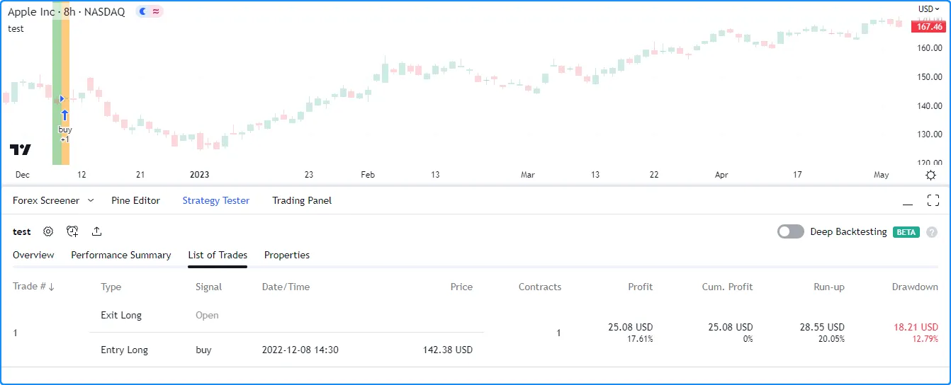
This example places a “buy” market order 100 bars before the last chart bar with strategy.entry(), then it attempts to cancel the order on the next bar with strategy.cancel_all(). The cancellation command does not affect the “buy” order because the broker emulator fills the order on the next bar’s opening tick, which occurs before the script evaluates the strategy.cancel_all() call:
Position sizing
Pine Script strategies feature two ways to control the sizes of the orders that open and manage positions:
- Set a default fixed quantity type and value for the orders. Programmers can specify defaults for these properties by including
default_qty_typeanddefault_qty_valuearguments in the strategy() declaration statement. Script users can adjust these values with the “Order size” inputs in the “Settings/Properties” tab. - Include a non-na
qtyargument in the strategy.entry() or strategy.order() call. When a call to either of these commands specifies a non-naqtyvalue, that call ignores the strategy’s default quantity type and value and places an order forqtycontracts/shares/lots/units instead.
The following example uses strategy.entry() calls with different qty values for long and short trades. When the current bar’s low equals the lowest value, the script places a “Buy” order to enter a long position of longAmount units. Otherwise, when the high equals the highest value, it places a “Sell” order to enter a short position of shortAmount units:
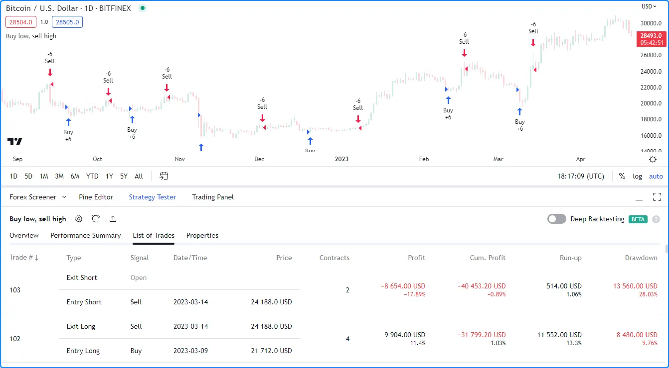
Notice that although we’ve included default_qty_type and default_qty_value arguments in the strategy() declaration statement, the strategy does not use this default setting to size its orders because the specified qty in the entry commands takes precedence. If we want to use the default size, we must remove the qty arguments from the strategy.entry() calls or set their values to na.
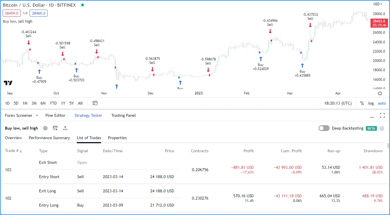
Here, we edited the previous script by including ternary expressions for the qty arguments in both strategy.entry() calls that replace input values of 0 with na. If the specified longAmount or shortAmount is 0, which is what we set as the new default, the corresponding entry orders use the strategy’s default order size instead, as we see below:
Closing a market position
By default, strategies close a market position using the First In, First Out (FIFO) method, which means that any exit order closes or reduces the position starting with the first open trade, even if the exit command specifies the entry ID of a different open trade. To override this default behavior, include close_entries_rule = "ANY" in the strategy() declaration statement.
The following example places “Buy1” and “Buy2” entry orders sequentially, starting 100 bars before the latest chart bar. When the position size is 0, it calls strategy.entry() to place the “Buy1” order for five units. After the strategy’s position size matches the size of that order, it uses strategy.entry() to place the “Buy2” order for ten units. The strategy then creates “bracket” exit orders for both entries using a single strategy.exit() call without a from_entry argument. For visual reference, the script plots the strategy.position_size value in a separate pane:
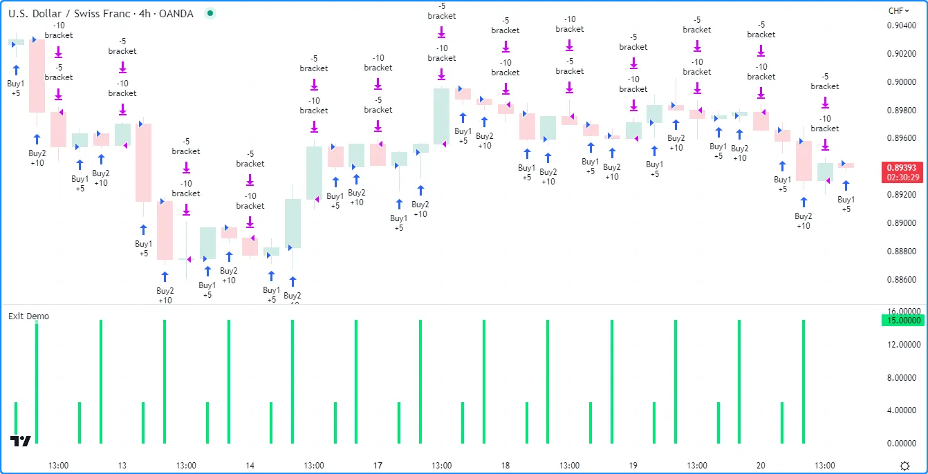
Note that:
- We included
pyramiding = 2in the strategy() declaration statement, allowing two successive entries from strategy.entry() per position.
Each time the market price triggers an exit order, the above script exits from the open position, starting with the oldest open trade. This FIFO behavior applies even if we explicitly specify an exit from “Buy2” before “Buy1” in the code.
The script version below calls strategy.close() with “Buy2” as its id argument, and it includes “Buy1” as the from_entry argument in the strategy.exit() call. The market order from strategy.close() executes on the next available tick, meaning the broker emulator fills it before the take-profit and stop-loss orders from strategy.exit():
The market order from the script’s strategy.close() call is for 10 units because it links to the open trade with the “Buy2” entry ID. A user might expect this strategy to close that trade completely when the order executes. However, the “List of Trades” tab shows that five units of the order go toward closing the “Buy1” trade first because it is the oldest, and the remaining five units close half of the “Buy2” trade. After that, the “bracket” orders from the strategy.exit() call close the rest of the position:
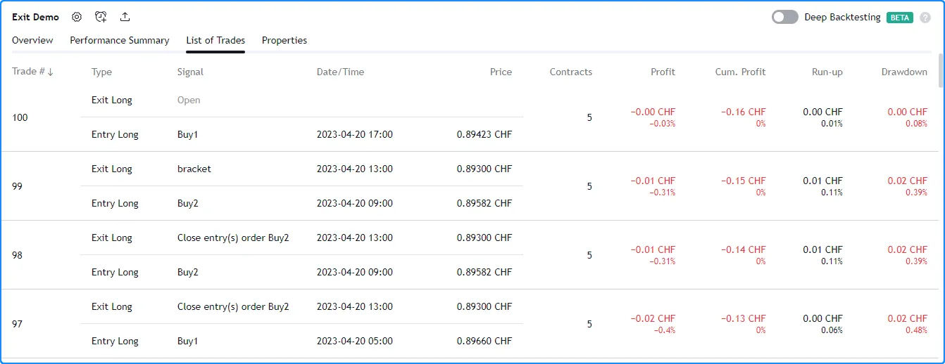
Note that:
- If we included
close_entries_rule = "ANY"in the strategy() declaration statement, the market order from strategy.close() would close the open trade with the “Buy2” entry ID first, and then the “bracket” orders from strategy.exit() would close the trade with the “Buy1” entry ID.
OCA groups
One-Cancels-All (OCA) groups allow a strategy to fully or partially cancel specific orders when the broker emulator executes another order from the same group. To assign an order to an OCA group, include an oca_name argument in the call to the order placement command. The strategy.entry() and strategy.order() commands also allow programmers to specify an OCA type, which defines whether a strategy cancels, reduces, or does not modify the order after executing other orders.
strategy.oca.cancel
When an order placement command uses strategy.oca.cancel as its oca_type argument, the strategy completely cancels the resulting order if another order from the same OCA group executes first.
To demonstrate how this OCA type impacts a strategy’s orders, consider the following script, which places orders when the ma1 value crosses the ma2 value. If the strategy.position_size is 0 when the cross occurs, the strategy places two stop orders with strategy.order() calls. The first is a long order at the bar’s high, and the second is a short order at the bar’s low. If the strategy already has an open position during the cross, it calls strategy.close_all() to close the position with a market order:
Depending on the price action, the strategy might fill both stop orders before creating the closing market order. In that case, the strategy exits the position without evaluating strategy.close_all() because both orders have the same size. We see this behavior in the chart below, where the strategy alternated between executing “Long” and “Short” orders a few times without executing an order from strategy.close_all():

To eliminate scenarios where the strategy fills the “Long” and “Short” orders before evaluating the strategy.close_all() call, we can instruct it to cancel one of the orders after it executes the other. Below, we included “Entry” as the oca_name argument and strategy.oca.cancel as the oca_type argument in both strategy.order() calls. Now, after the strategy executes either the “Long” or “Short” order, it cancels the other order and waits for strategy.close_all() to close the position:

strategy.oca.reduce
When an order placement command uses strategy.oca.reduce as its OCA type, the strategy does not cancel the resulting order entirely if another order with the same OCA name executes first. Instead, it reduces the order’s size by the filled number of contracts/shares/lots/units, which is particularly useful for custom exit strategies.
The following example demonstrates a long-only strategy that generates a single stop-loss order and two take-profit orders for each new entry. When a faster moving average crosses over a slower one, the script calls strategy.entry() with qty = 6 to create an entry order, and then it uses three strategy.order() calls to create a stop order at the stop price and two limit orders at the limit1 and limit2 prices. The strategy.order() call for the “Stop” order uses qty = 6, and the two calls for the “Limit 1” and “Limit 2” orders both use qty = 3:
After adding this strategy to the chart, we see it does not work as initially intended. The problem with this script is that the orders from strategy.order() do not belong to an OCA group by default (unlike strategy.exit(), whose orders automatically belong to a strategy.oca.reduce OCA group). Since the strategy does not assign the strategy.order() calls to any OCA group, it does not reduce any unfilled stop or limit orders after executing an order. Consequently, if the broker emulator fills the stop order and at least one of the limit orders, the traded quantity exceeds the open long position, resulting in an open short position:
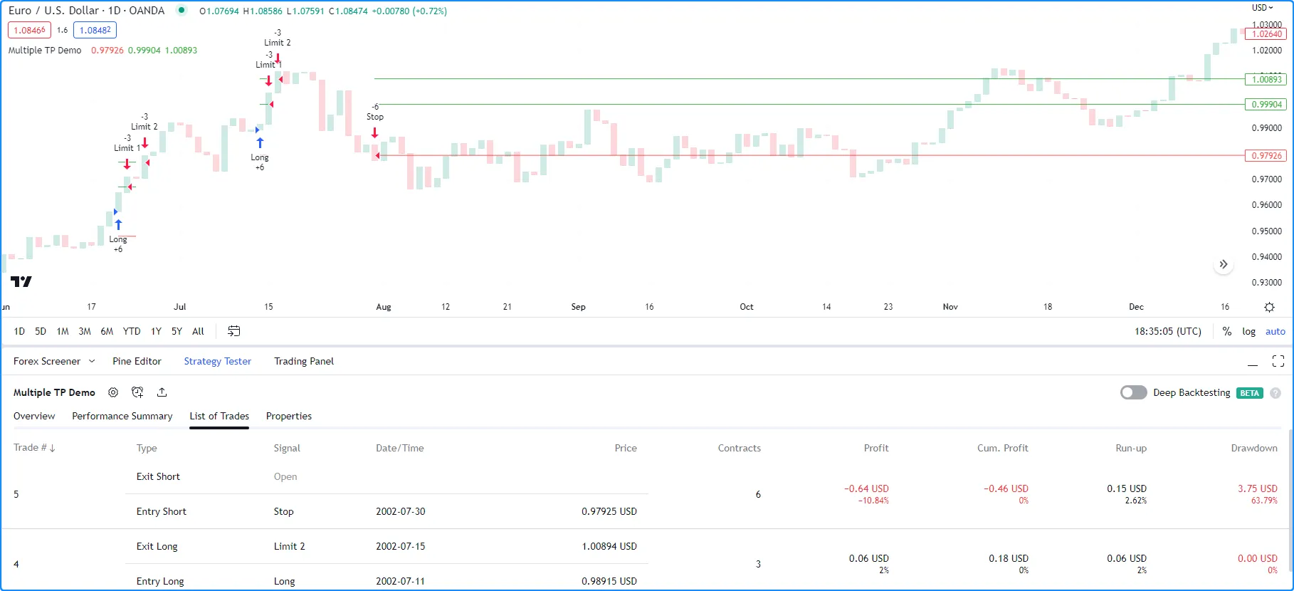
For our long-only strategy to work as we intended, we must instruct it to reduce the sizes of the unfilled stop/limit orders after one of them executes to prevent selling a larger quantity than the open long position.
Below, we specified “Bracket” as the oca_name and strategy.oca.reduce as the oca_type in all the script’s strategy.order() calls. These changes tell the strategy to reduce the sizes of the orders in the “Bracket” group each time the broker emulator fills one of them. This version of the strategy never simulates a short position because the total size of its filled stop and limit orders never exceeds the long position’s size:
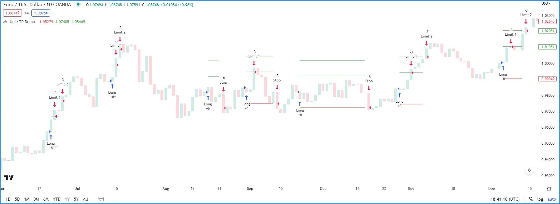
Note that:
- We also changed the
qtyvalue of the “Limit 2” order to 6 instead of 3 because the strategy reduces its amount by three units when it executes the “Limit 1” order. Keeping theqtyvalue of 3 would cause the second limit order’s size to drop to 0 after the strategy fills the first limit order, meaning it would never execute.
strategy.oca.none
When an order placement command uses strategy.oca.none as its oca_type value, all orders from that command execute independently of any OCA group. This value is the default oca_type for the strategy.order() and strategy.entry() commands.
Currency
Pine Script strategies can use different currencies in their calculations than the instruments they simulate trades on. Programmers can specify a strategy’s account currency by including a currency.* variable as the currency argument in the strategy() declaration statement. The default value is currency.NONE, meaning the strategy uses the same currency as the current chart (syminfo.currency). Script users can change the account currency using the “Base currency” input in the script’s “Settings/Properties” tab.
When a strategy script uses an account currency that differs from the chart’s currency, it uses the previous daily value of a corresponding currency pair from the most popular exchange to determine the conversion rate. If no exchange provides the rate directly, it derives the rate using a spread symbol. The strategy multiplies all monetary values, including simulated profits/losses, by the determined cross rate to express them in the account currency. To retrieve the rate that a strategy uses to convert monetary values, call request.currency_rate() with syminfo.currency as the from argument and strategy.account_currency as the to argument.
Note that:
- Programmers can directly convert values expressed in a strategy’s account currency to the chart’s currency and vice versa via the strategy.convert_to_symbol() and strategy.convert_to_account() functions.
The following example demonstrates how currency conversion affects a strategy’s monetary values and how a strategy’s cross-rate calculations match those that request.*() functions use.
On each of the latest 500 bars, the strategy places an entry order with strategy.entry(), and it places a take-profit and stop-loss order one tick away from the entry price with strategy.exit(). The size of each entry order is 1.0 / syminfo.mintick, rounded to the nearest tick, which means that the profit/loss of each closed trade is equal to one point in the chart’s quote currency. We specified currency.EUR as the account currency in the strategy() declaration statement, meaning the strategy multiplies all monetary values by a cross rate to express them in Euros.
The script calculates the absolute change in the ratio of the strategy’s net profit (strategy.netprofit) to the symbol’s point value (syminfo.pointvalue) to determine the value of one unit of the chart’s currency in Euros. It plots this value alongside the result from a request.currency_rate() call that uses syminfo.currency and strategy.account_currency as the from and to arguments. As we see below, both plots align, confirming that strategies and request.*() functions use the same daily cross-rate calculations:
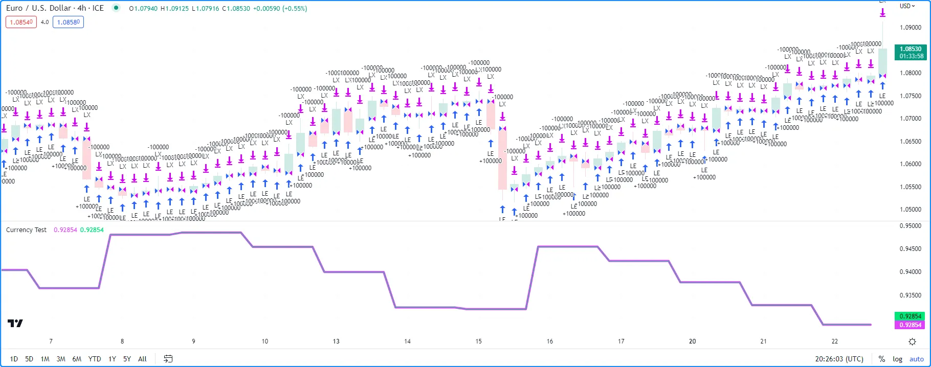
Note that:
- When a strategy executes on a chart with a timeframe higher than “1D”, it uses the data from one day before each historical bar’s closing time for its cross-rate calculations. For example, on a “1W” chart, the strategy bases its cross rate on the previous Thursday’s closing values. However, it still uses the latest confirmed daily rate on realtime bars.
Altering calculation behavior
Strategy scripts execute across all available historical chart bars and continue to execute on realtime bars as new data comes in. However, by default, strategies only recalculate their values after a bar closes, even on realtime bars, and the earliest point that the broker emulator fills the orders a strategy places on the close one bar is at the open of the following bar.
Users can change these behaviors with the calc_on_every_tick, calc_on_order_fills, and process_orders_on_close parameters of the strategy() declaration statement or the corresponding inputs in the “Recalculate” and “Fill orders” sections of the script’s “Settings/Properties” tab. The sections below explain how these settings affect a strategy’s calculations.
calc_on_every_tick
The calc_on_every_tick parameter of the strategy() function determines the frequency of a strategy’s calculations on realtime bars. When this parameter’s value is true, the script recalculates on each new tick in the realtime data feed. Its default value is false, meaning the script only executes on a realtime bar after it closes. Users can also toggle this recalculation behavior with the “On every tick” input in the script’s “Settings/Properties” tab.
Enabling this setting can be useful in forward testing because it allows a strategy to use realtime price updates in its calculations. However, it does not affect the calculations on historical bars because historical data feeds do not contain complete tick data: the broker emulator considers each historical bar to have only four ticks (open, high, low, and close). Therefore, users should exercise caution and understand the limitations of this setting. If enabling calculation on every tick causes a strategy to behave differently on historical and realtime bars, the strategy will repaint after the user reloads it.
The following example demonstrates how recalculation on every tick can cause strategy repainting. The script uses strategy.entry() calls to place a long entry order each time the close reaches its highest value and a short entry order each time the close reaches its lowest value. The strategy() declaration statement includes calc_on_every_tick = true, meaning that on realtime bars, it can recalculate and place orders on new price updates before a bar closes:
Note that:
- The script uses a pyramiding value of 20, allowing it to simulate up to 20 entries per position with the strategy.entry() command.
- The script highlights the chart’s background orange when barstate.isrealtime is
trueto indicate realtime bars.
After applying the script to our chart and letting it run on several realtime bars, we see the following output:
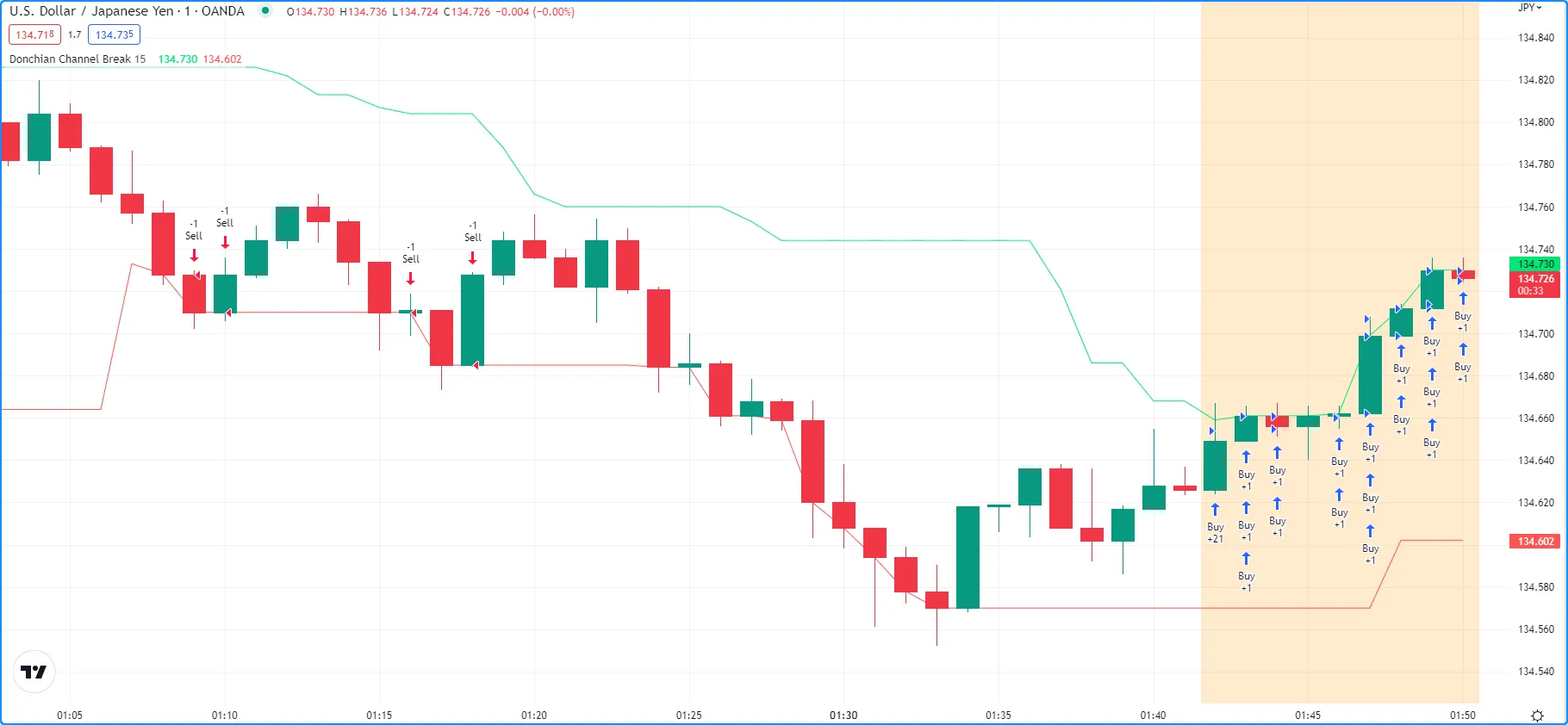
The script placed a “Buy” order on each tick where the close was at the highest value, which happened more than once on each realtime bar. Additionally, the broker emulator filled each market order at the current realtime price rather than strictly at the open of the following chart bar.
After we reload the chart, we see that the strategy changed its behavior and repainted its results on those bars. This time, the strategy placed only one “Buy” order for each closed bar where the condition was valid, and the broker emulator filled each order at the open of the following bar. It did not generate multiple entries per bar because what were previously realtime bars became historical bars, which do not hold complete tick data:
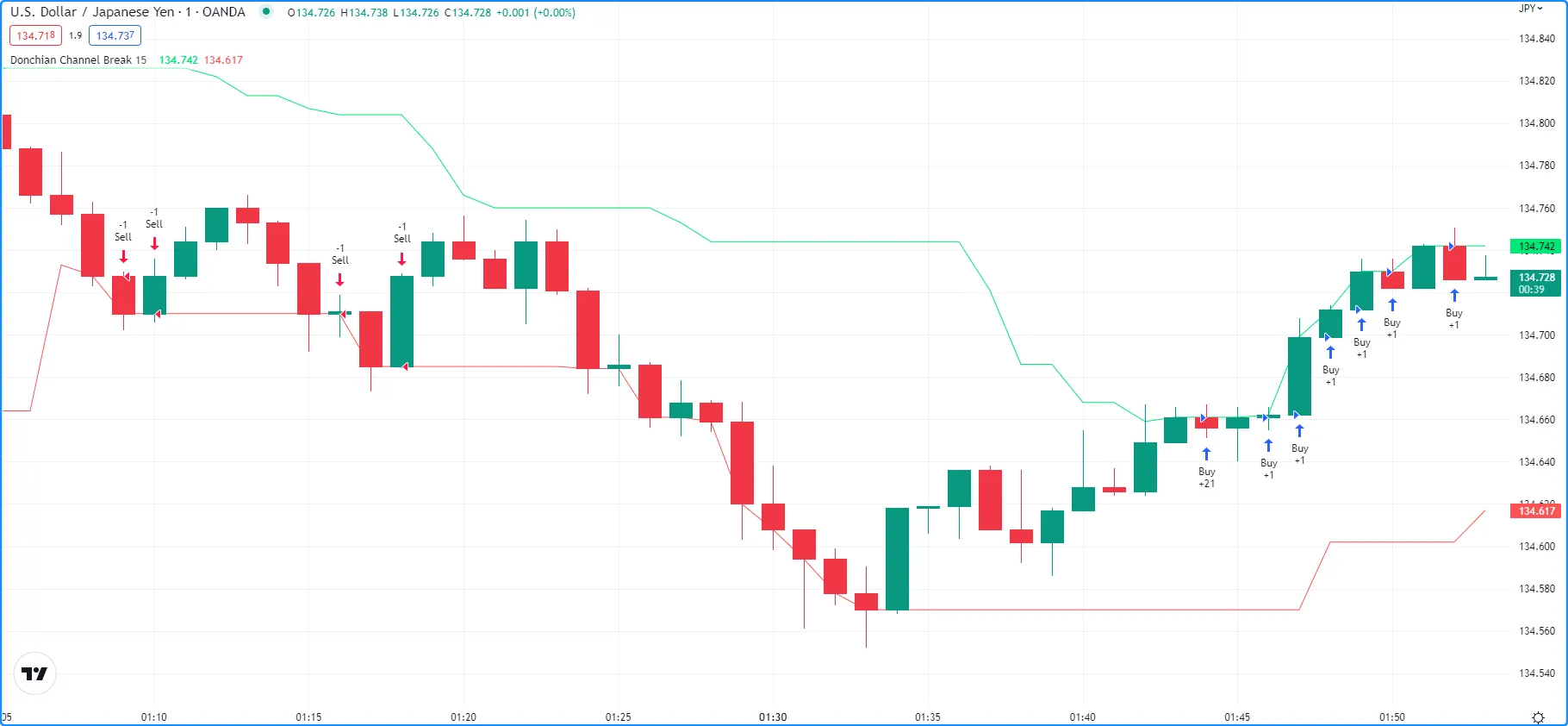
calc_on_order_fills
The calc_on_order_fills parameter of the strategy() function enables a strategy to recalculate immediately after an order fills, allowing it to use more granular information and place additional orders without waiting for a bar to close. Its default value is false, meaning the strategy does not allow recalculation immediately after every order fill. Users can also toggle this behavior with the “After order is filled” input in the script’s “Settings/Properties” tab.
Enabling this setting can provide a strategy script with additional data that would otherwise not be available until after a bar closes, such as the current average price of a simulated position on an open bar.
The example below shows a simple strategy that creates a “Buy” order with strategy.entry() whenever the strategy.position_size is 0. The script uses strategy.position_avg_price to calculate price levels for the strategy.exit() call’s stop-loss and take-profit orders that close the position.
We’ve included calc_on_order_fills = true in the strategy() declaration statement, meaning that the strategy recalculates each time the broker emulator fills a “Buy” or “Exit” order. Each time an “Exit” order fills, the strategy.position_size reverts to 0, triggering a new “Buy” order. The broker emulator fills the “Buy” order on the next tick at one of the bar’s OHLC values, and then the strategy uses the recalculated strategy.position_avg_price value to determine new “Exit” order prices:
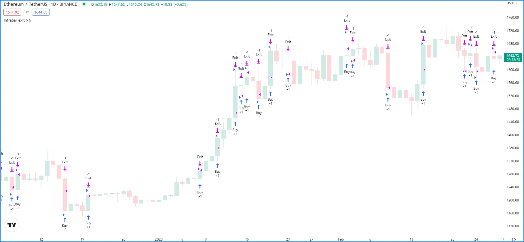
Note that:
- Without enabling recalculation on order fills, this strategy would not place new orders before a bar closes. After an exit, the strategy would wait for the bar to close before placing a new “Buy” order, which the broker emulator would fill on the next tick after that, i.e., the open of the following bar.
It’s important to note that enabling calc_on_order_fills can produce unrealistic strategy results in some cases because the broker emulator may assume order-fill prices that are not obtainable in real-world trading. Therefore, users should exercise caution and carefully examine their strategy logic when allowing recalculation on order fills.
For example, the following script places a “Buy” order after each new order fill and bar close over the most recent 25 historical bars. The strategy simulates four entries per bar because the broker emulator considers each historical bar to have four ticks (open, high, low, and close). This behavior is unrealistic because it is not typically possible to fill an order at a bar’s exact high or low price:

process_orders_on_close
By default, strategies simulate orders at the close of each bar, meaning that the earliest opportunity to fill the orders and execute strategy calculations and alerts is on the opening of the following bar. Programmers can change this behavior to process orders on the closing tick of each bar by setting process_orders_on_close to true in the strategy() declaration statement. Users can set this behavior by changing the “Fill Orders/On Bar Close” setting in the “Settings/Properties” tab.
This behavior is most useful when backtesting manual strategies in which traders exit from a position before a bar closes, or in scenarios where algorithmic traders in non-24x7 markets set up after-hours trading capability so that alerts sent after close still have hope of filling before the following day.
Note that:
- Using strategies with
process_orders_on_closeenabled to send alerts to a third-party service might cause unintended results. Alerts on the close of a bar still occur after the market closes, and real-world orders based on such alerts might not fill until after the market opens again. - The strategy.close() and strategy.close_all() commands feature an
immediatelyparameter that, iftrue, allows the resulting market order to fill on the same tick where the strategy created it. This parameter provides an alternative way for programmers to selectively applyprocess_orders_on_closebehavior to closing market orders without affecting the behavior of other order placement commands.
Simulating trading costs
Strategy performance reports are more relevant and meaningful when they include potential real-world trading costs. Without modeling the potential costs associated with their trades, traders may overestimate a strategy’s historical profitability, potentially leading to suboptimal decisions in live trading. Pine Script strategies include inputs and parameters for simulating trading costs in performance results.
Commission
Commission is the fee a broker/exchange charges when executing trades. Commission can be a flat fee per trade or contract/share/lot/unit, or a percentage of the total transaction value. Users can set the commission properties of their strategies by including commission_type and commission_value arguments in the strategy() function, or by setting the “Commission” inputs in the “Properties” tab of the strategy settings.
The following script is a simple strategy that simulates a “Long” position of 2% of equity when close equals the highest value over the length, and closes the trade when it equals the lowest value:
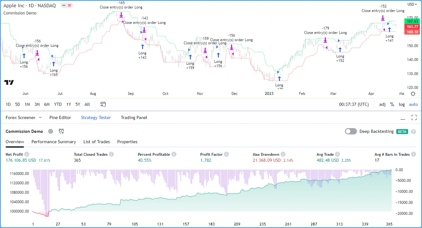
The results in the Strategy Tester show that the strategy had a positive equity growth of 17.61% over the testing range. However, the backtest results do not account for fees the broker/exchange may charge. Let’s see what happens to these results when we include a small commission on every trade in the strategy simulation. In this example, we’ve included commission_type = strategy.commission.percent and commission_value = 1 in the strategy() declaration, meaning it will simulate a commission of 1% on all executed orders:
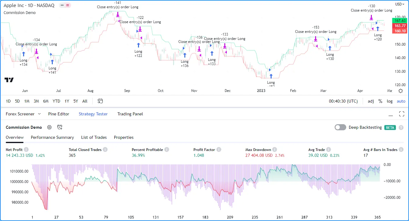
As we can see in the example above, after applying a 1% commission to the backtest, the strategy simulated a significantly reduced net profit of only 1.42% and a more volatile equity curve with an elevated max drawdown. These results highlight the impact that commission can have on a strategy’s hypothetical performance.
Slippage and unfilled limits
In real-life trading, a broker/exchange may fill orders at slightly different prices than a trader intended, due to volatility, liquidity, order size, and other market factors, which can profoundly impact a strategy’s performance. The disparity between expected prices and the actual prices at which the broker/exchange executes trades is what we refer to as slippage. Slippage is dynamic and unpredictable, making it impossible to simulate precisely. However, factoring in a small amount of slippage on each trade during a backtest or forward test might help the results better align with reality. Users can model slippage in their strategy results, sized as a fixed number of ticks, by including a slippage argument in the strategy() declaration statement or by setting the “Slippage” input in the “Settings/Properties” tab.
The following example demonstrates how simulating slippage affects the fill prices of market orders in a strategy test. The script below places a “Buy” market order of 2% equity when the market price is above a rising EMA and closes the position when the price dips below the EMA while it’s falling. We’ve included slippage = 20 in the strategy() function, which declares that the price of each simulated order will slip 20 ticks in the direction of the trade.
The script uses strategy.opentrades.entry_bar_index() and strategy.closedtrades.exit_bar_index() to get the entryIndex and exitIndex, which it uses to obtain the fillPrice of the order. When the bar index is at the entryIndex, the fillPrice is the first strategy.opentrades.entry_price() value. At the exitIndex, fillPrice is the strategy.closedtrades.exit_price() value from the last closed trade. The script plots the expected fill price along with the simulated fill price after slippage to visually compare the difference:
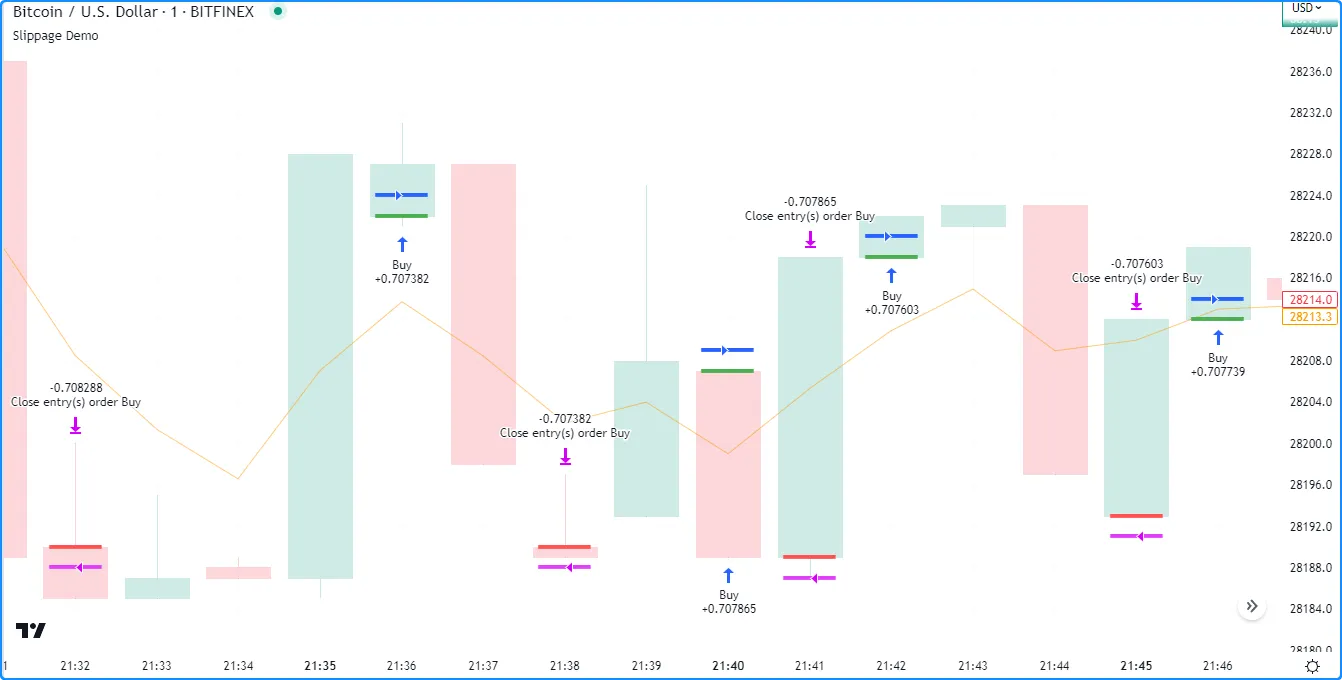
Note that:
- Since the strategy applies constant slippage to all order fills, some orders can fill outside the candle range in the simulation. Exercise caution with this setting, as adding excessive simulated slippage can produce unrealistically worse testing results.
Some traders might assume that they can avoid the adverse effects of slippage by using limit orders, as unlike market orders, they cannot execute at a worse price than the specified value. However, even if the market price reaches an order’s price, there’s a chance that a limit order might not fill, depending on the state of the real-life market, because limit orders can only fill if a security has sufficient liquidity and price action around their values. To account for the possibility of unfilled orders in a backtest, users can specify the backtest_fill_limits_assumption value in the declaration statement or use the “Verify price for limit orders” input in the “Settings/Properties” tab. This setting instructs the strategy to fill limit orders only after the market price moves a defined number of ticks past the order prices.
The following example places a limit order of 2% equity at a bar’s hlcc4 price when the high is the highest value over the past length bars and there are no pending entries. The strategy closes the market position and cancels all orders after the low is the lowest value. Each time the strategy triggers an order, it draws a horizontal line at the limitPrice, which it updates on each bar until closing the position or canceling the order:
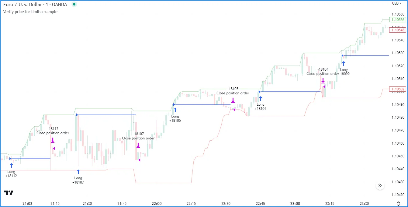
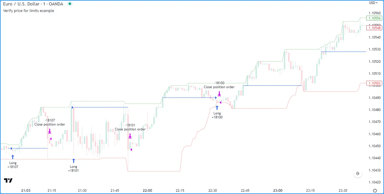
By default, the script assumes that all limit orders are guaranteed to fill when the market price reaches their values, which is often not the case in real-life trading. Let’s add price verification to our limit orders to account for potentially unfilled ones. In this example, we’ve included backtest_fill_limits_assumption = 3 in the strategy() function call. As we can see, using limit verification omits some simulated order fills and changes the times of others, because the entry orders can now only fill after the price exceeds the limit price by three ticks:
Risk management
Designing a strategy that performs well, especially in a broad class of markets, is a challenging task. Most strategies are designed for specific market patterns/conditions and can produce uncontrolled losses when applied to other data. Therefore, a strategy’s risk management behavior can be critical to its performance. Programmers can set risk management criteria in their strategy scripts using the strategy.risk.*() commands.
Strategies can incorporate any number of risk management criteria in any combination. All risk management commands execute on every tick and order execution event, regardless of any changes to the strategy’s calculation behavior. There is no way to deactivate any of these commands on specific script executions. Irrespective of a risk management command’s location, it always applies to the strategy unless the programmer removes the call from the code.
strategy.risk.allow_entry_in()
strategy.risk.max_cons_loss_days()
strategy.risk.max_intraday_filled_orders()
strategy.risk.max_intraday_loss()
strategy.risk.max_position_size()
Margin
Margin is the minimum percentage of a market position that a trader must hold in their account as collateral to receive and sustain a loan from their broker to achieve their desired leverage. The margin_long and margin_short parameters of the strategy() declaration statement and the “Margin for long/short positions” inputs in the “Properties” tab of the script settings specify margin percentages for long and short positions. For example, if a trader sets the margin for long positions to 25%, they must have enough funds to cover 25% of an open long position. This margin percentage also means the trader can potentially spend up to 400% of their equity on their trades.
If a strategy’s simulated funds cannot cover the losses from a margin trade, the broker emulator triggers a margin call, which forcibly liquidates all or part of the open position. The exact number of contracts/shares/lots/units that the emulator liquidates is four times the amount required to cover the loss, which helps prevent constant margin calls on subsequent bars. The emulator determines liquidated quantity using the following algorithm:
- Calculate the amount of capital spent on the position:
Money Spent = Quantity * Entry Price - Calculate the Market Value of Security (MVS):
MVS = Position Size * Current Price - Calculate the Open Profit as the difference between
MVSandMoney Spent. If the position is short, multiply this value by -1. - Calculate the strategy’s equity value:
Equity = Initial Capital + Net Profit + Open Profit - Calculate the margin ratio:
Margin Ratio = Margin Percent / 100 - Calculate the margin value, which is the cash required to cover the hypothetical account’s portion of the position:
Margin = MVS * Margin Ratio - Calculate the strategy’s available funds:
Available Funds = Equity - Margin - Calculate the total amount of money lost:
Loss = Available Funds / Margin Ratio - Calculate the number of contracts/shares/lots/units the account must liquidate to cover the loss, truncated to the same decimal precision as the minimum position size for the current symbol:
Cover Amount = TRUNCATE(Loss / Current Price). - Multiply the quantity required to cover the loss by four to determine the margin call size:
Margin Call Size = Cover Amount * 4
To examine this calculation in detail, let’s add the built-in Supertrend Strategy to the NASDAQ:TSLA chart on the “1D” timeframe and set the “Order size” to 300% of equity and the “Margin for long positions” to 25% in the “Properties” tab of the strategy settings:
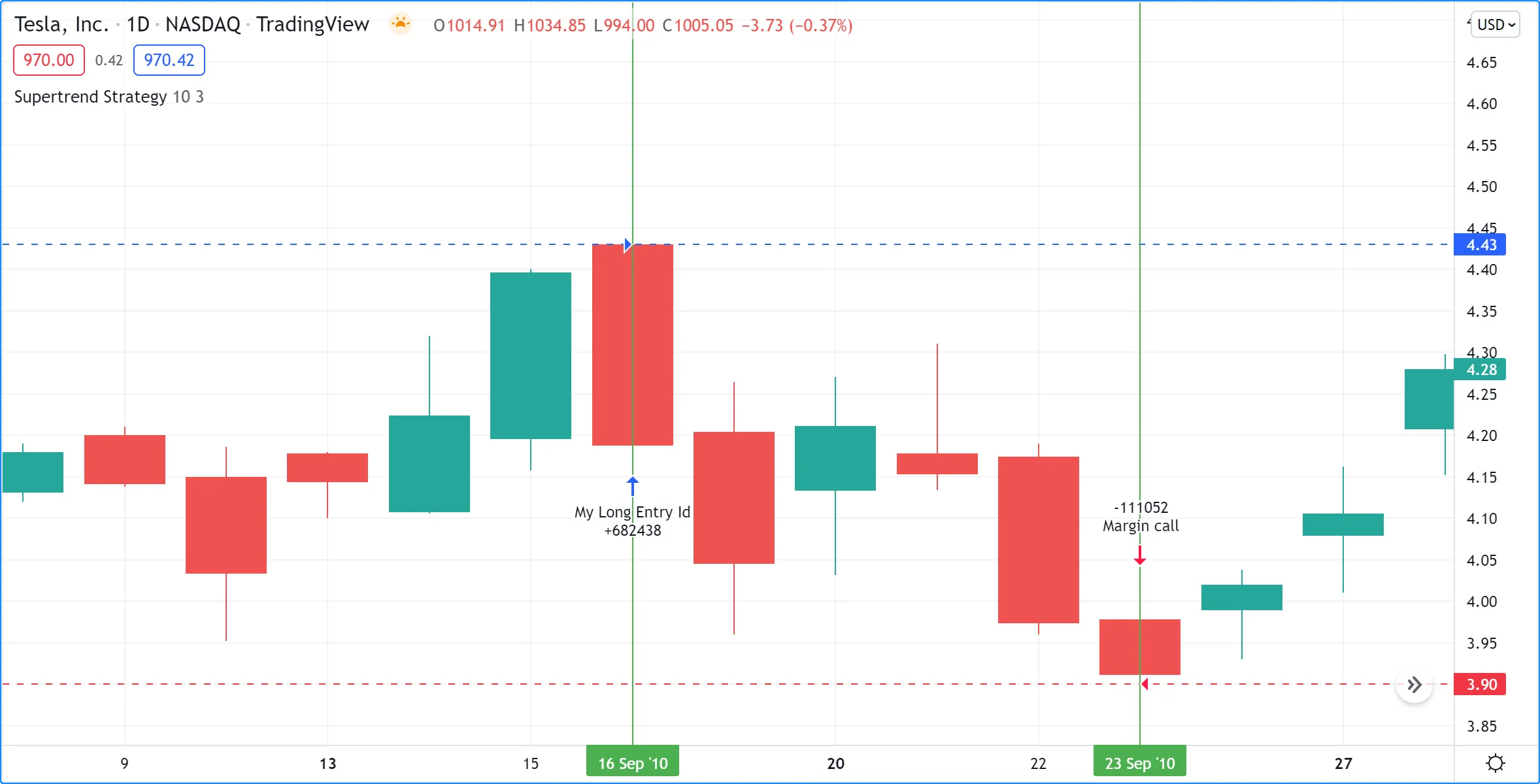
The first entry happened at the bar’s opening price on 16 Sep 2010. The strategy bought 682,438 shares (Position Size) at 4.43 USD (Entry Price). Then, on 23 Sep 2010, when the price dipped to 3.9 (Current Price), the emulator forcibly liquidated 111,052 shares with a margin call. The calculations below show how the broker emulator determined this amount for the margin call event:
Money spent: 682438 * 4.43 = 3023200.34MVS: 682438 * 3.9 = 2661508.2Open Profit: −361692.14Equity: 1000000 + 0 − 361692.14 = 638307.86Margin Ratio: 25 / 100 = 0.25Margin: 2661508.2 * 0.25 = 665377.05Available Funds: 638307.86 - 665377.05 = -27069.19Money Lost: -27069.19 / 0.25 = -108276.76Cover Amount: TRUNCATE(-108276.76 / 3.9) = TRUNCATE(-27763.27) = -27763Margin Call Size: -27763 * 4 = - 111052Note that:
- The strategy.margin_liquidation_price variable’s value represents the price level that will cause a margin call if the market price reaches it. For more information about how margin works and the formula for calculating a position’s margin call price, see this page in our Help Center.
Using strategy information in scripts
Numerous built-ins within the strategy.* namespace and its sub-namespaces provide convenient solutions for programmers to use a strategy’s trade and performance information, including data shown in the Strategy Tester, directly within their code’s logic and calculations.
Several strategy.* variables hold fundamental information about a strategy, including its starting capital, equity, profits and losses, run-up and drawdown, and open position:
- strategy.account_currency
- strategy.initial_capital
- strategy.equity
- strategy.netprofit and strategy.netprofit_percent
- strategy.grossprofit and strategy.grossprofit_percent
- strategy.grossloss and strategy.grossloss_percent
- strategy.openprofit and strategy.openprofit_percent
- strategy.max_runup and strategy.max_runup_percent
- strategy.max_drawdown and strategy.max_drawdown_percent
- strategy.position_size
- strategy.position_avg_price
- strategy.position_entry_name
Additionally, the namespace features multiple variables that hold general trade information, such as the number of open and closed trades, the number of winning and losing trades, average trade profits, and maximum trade sizes:
- strategy.opentrades
- strategy.closedtrades
- strategy.wintrades
- strategy.losstrades
- strategy.eventrades
- strategy.avg_trade and strategy.avg_trade_percent
- strategy.avg_winning_trade and strategy.avg_winning_trade_percent
- strategy.avg_losing_trade and strategy.avg_losing_trade_percent
- strategy.max_contracts_held_all
- strategy.max_contracts_held_long
- strategy.max_contracts_held_short
Programmers can use these variables to display relevant strategy information on their charts, create customized trading logic based on strategy data, calculate custom performance metrics, and more.
The following example demonstrates a few simple use cases for these strategy.* variables. The script uses them in its order placement and display calculations. When the calculated rank crosses above 10 and the strategy.opentrades value is 0, the script calls strategy.entry() to place a “Buy” market order. On the following bar, where that order fills, it calls strategy.exit() to create a stop-loss order at a user-specified percentage below the strategy.position_avg_price value. If the rank crosses above 80 during the open trade, the script uses strategy.close() to exit the position on the next bar.
The script creates a table to display formatted strings representing information from several of the above strategy.* variables on the main chart pane. The text in the table shows the strategy’s net profit and net profit percentage, the account currency, the number of winning trades and the win percentage, the ratio of the average winning trade to the average losing trade, and the profit factor (the ratio of the gross profit to the gross loss). The script also plots the strategy.equity series in a separate pane and highlights the pane’s background based on the value of strategy.openprofit:
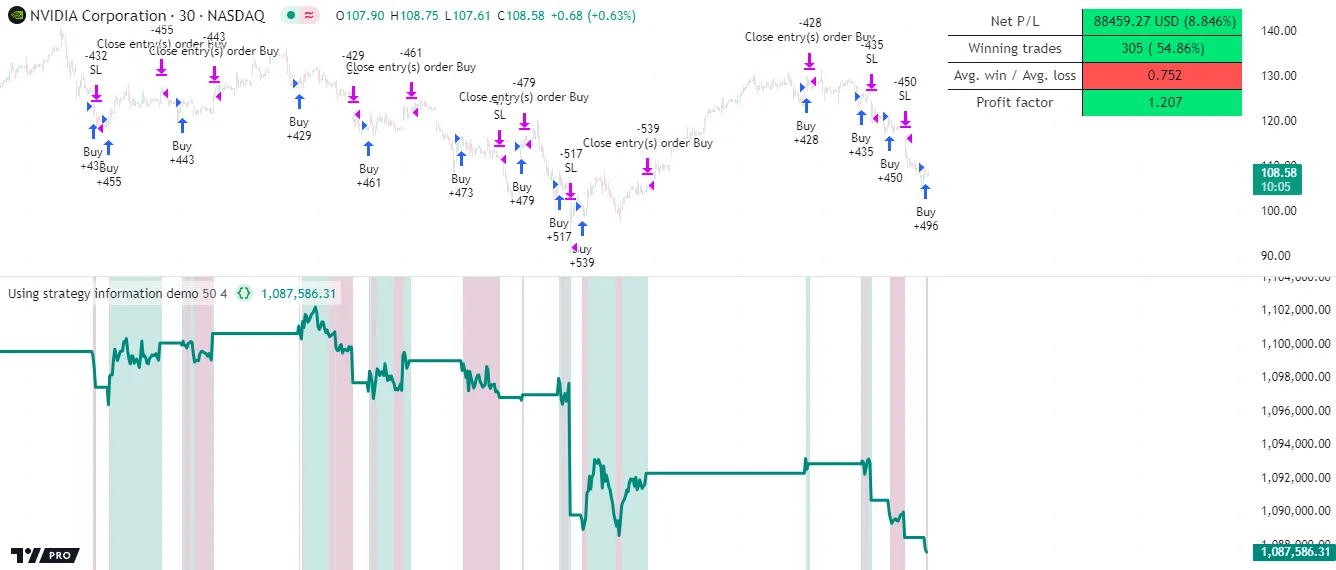
Note that:
- This script creates a stop-loss order one bar after the entry order because it uses strategy.position_avg_price to determine the price level. This variable has a non-na value only when the strategy has an open position.
- The script draws the table only on the last historical bar and all realtime bars because the historical states of tables are never visible. See the Reducing drawing updates section of the Profiling and optimization page for more information.
- The table.new() call includes
force_overlay = trueto display the table on the main chart pane.
Individual trade information
The strategy.* namespace features two sub-namespaces that provide access to individual trade information: strategy.opentrades.* and strategy.closedtrades.*. The strategy.opentrades.* built-ins return data for incomplete (open) trades, and the strategy.closedtrades.* built-ins return data for completed (closed) trades. With these built-ins, programmers can use granular trade data in their scripts, allowing for more detailed strategy analysis and advanced calculations.
Both sub-namespaces contain several similar functions that return information about a trade’s orders, simulated costs, and profit/loss, including:
- strategy.opentrades.entry_id() / strategy.closedtrades.entry_id()
- strategy.opentrades.entry_price() / strategy.closedtrades.entry_price()
- strategy.opentrades.entry_bar_index() / strategy.closedtrades.entry_bar_index()
- strategy.opentrades.entry_time() / strategy.closedtrades.entry_time()
- strategy.opentrades.entry_comment() / strategy.closedtrades.entry_comment()
- strategy.opentrades.size() / strategy.closedtrades.size()
- strategy.opentrades.profit() / strategy.closedtrades.profit()
- strategy.opentrades.profit_percent() / strategy.closedtrades.profit_percent()
- strategy.opentrades.commission() / strategy.closedtrades.commission()
- strategy.opentrades.max_runup() / strategy.closedtrades.max_runup()
- strategy.opentrades.max_runup_percent() / strategy.closedtrades.max_runup_percent()
- strategy.opentrades.max_drawdown() / strategy.closedtrades.max_drawdown()
- strategy.opentrades.max_drawdown_percent() / strategy.closedtrades.max_drawdown_percent()
- strategy.closedtrades.exit_id()
- strategy.closedtrades.exit_price()
- strategy.closedtrades.exit_time()
- strategy.closedtrades.exit_bar_index()
- strategy.closedtrades.exit_comment()
Note that:
- Most built-ins within these namespaces are functions. However, the
strategy.opentrades.*namespace also features a unique variable: strategy.opentrades.capital_held. Its value represents the amount of capital reserved by all open trades. - Only the
strategy.closedtrades.*namespace has.exit_*()functions that return information about exit orders.
All strategy.opentrades.*() and strategy.closedtrades.*() functions have a trade_num parameter, which accepts an “int” value representing the index of the open or closed trade. The index of the first open/closed trade is 0, and the last trade’s index is one less than the value of the strategy.opentrades/strategy.closedtrades variable.
The following example places up to five long entry orders per position, each with a unique ID, and it calculates metrics for specific closed trades.
The strategy places a new entry order when the close crosses above the median value without reaching the highest value, but only if the number of open trades is less than five. It exits each position using stop-loss orders from strategy.exit() or a market order from strategy.close_all(). Each successive entry order’s ID depends on the number of open trades. The first entry ID in each position is "Buy0", and the last possible entry ID is "Buy4".
The script calls strategy.closedtrades.*() functions within a for loop to access closed trade entry IDs, profits, entry bar indices, and exit bar indices. It uses this information to calculate the total number of closed trades with the specified entry ID, the number of winning trades, the average number of bars per trade, and the total profit from all the trades. The script then organizes this information in a formatted string and displays the result using a single-cell table:
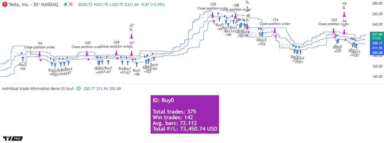
Note that:
- This strategy can open up to five long trades per position because we included
pyramiding = 5in the strategy() declaration statement. See the pyramiding section for more information. - The strategy.exit() instance in this script persists and generates exit orders for every entry in the open position because we did not specify a
from_entryID. See the Exits for multiple entries section to learn more about this behavior.
Strategy alerts
Pine Script indicators (not strategies) have two different mechanisms to set up custom alert conditions: the alertcondition() function, which tracks one specific condition per function call, and the alert() function, which tracks all its calls simultaneously, but provides greater flexibility in the number of calls, alert messages, etc.
Pine Script strategies cannot create alert triggers using the alertcondition() function, but they can create triggers with the alert() function. Additionally, each order placement command comes with its own built-in alert functionality that does not require any additional code to implement. As such, any strategy that uses an order placement command can issue alerts upon order execution. The precise mechanics of such built-in strategy alerts are described in the Order Fill events section of the Alerts page.
When a strategy uses both the alert() function and functions that create orders in the same script, the “Create Alert” dialog box provides a choice between the conditions to use as a trigger: alert() events, order fill events, or both.
For many trading strategies, the delay between a triggered alert and a live trade can be a critical performance factor. By default, strategy scripts can only execute alert() function calls on the close of realtime bars, as if they used alert.freq_once_per_bar_close, regardless of the freq argument in the call. Users can change the alert frequency by including calc_on_every_tick = true in the strategy() call or selecting the “Recalculate/On every tick” option in the “Settings/Properties” tab before creating the alert. However, depending on the script, this setting can adversely impact the strategy’s behavior. See the `calc_on_every_tick` section for more information.
Order fill alert triggers do not suffer the same limitations as the triggers from alert() calls, which makes them more suitable for sending alerts to third parties for automation. Alerts from order fill events execute immediately, unaffected by a script’s calc_on_every_tick setting. Users can set the default message for order fill alerts via the //@strategy_alert_message compiler annotation. The text provided with this annotation populates the “Message” field in the “Create Alert” dialog box.
The following script shows a simple example of a default order fill alert message. Above the strategy() declaration statement, the script includes @strategy_alert_message with placeholders for the trade action, current position size, ticker name, and fill price values in the message text:
This script populates the “Create Alert” dialog box with its default message when the user selects its name from the “Condition” dropdown tab:
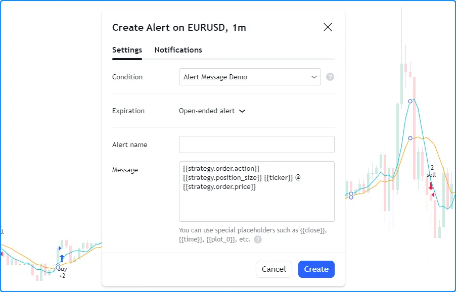
When the alert fires, the strategy populates the placeholders in the alert message with their corresponding values. For example:
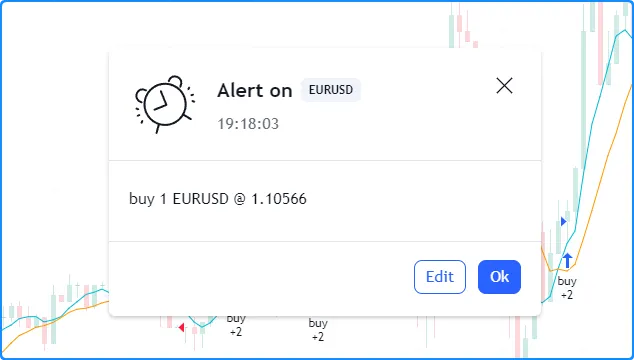
Notes on testing strategies
Testing and tuning strategies in historical and live market conditions can provide insight into a strategy’s characteristics, potential weaknesses, and possibly its future potential. However, traders should always be aware of the biases and limitations of simulated strategy results, especially when using the results to support live trading decisions. This section outlines some caveats associated with strategy validation and tuning and possible solutions to mitigate their effects.
Backtesting and forward testing
Backtesting is a technique to evaluate the historical performance of a trading strategy or model by simulating and analyzing its past results on historical market data. This technique assumes that a strategy’s results on past data can provide insight into its strengths and weaknesses. When backtesting, many traders adjust the parameters of a strategy in an attempt to optimize its results. Analysis and optimization of historical results can help traders to gain a deeper understanding of a strategy. However, traders should always understand the risks and limitations when basing their decisions on optimized backtest results.
It is prudent to also use realtime analysis as a tool for evaluating a trading system on a forward-looking basis. Forward testing aims to gauge the performance of a strategy in live market conditions, where factors such as trading costs, slippage, and liquidity can meaningfully affect its performance. While forward testing has the distinct advantage of not being affected by certain types of biases (e.g., lookahead bias or “future data leakage”), it does carry the disadvantage of being limited in the quantity of data to test. Therefore, although it can provide helpful insights into a strategy’s performance in current market conditions, forward testing is not typically used on its own.
Lookahead bias
One typical issue in backtesting strategies that request alternate timeframe data, use repainting variables such as timenow, or alter calculation behavior for intrabar order fills, is the leakage of future data into the past during evaluation, which is known as lookahead bias. Not only is this bias a common cause of unrealistic strategy results, since the future is never actually knowable beforehand, but it is also one of the typical causes of strategy repainting.
Traders can often confirm whether a strategy has lookahead bias by forward testing it on realtime data, where no known data exists beyond the latest bar. Since there is no future data to leak into the past on realtime bars, the strategy will behave differently on historical and realtime bars if its results have lookahead bias.
To eliminate lookahead bias in a strategy:
- Do not use repainting variables that leak future values into the past in the order placement or cancellation logic.
- Do not include barmerge.lookahead_on in
request.*()calls without offsetting the data series, as described in this section of the Repainting page. - Use realistic strategy calculation behavior.
Selection bias
Selection bias occurs when a trader analyzes only results on specific instruments or timeframes while ignoring others. This bias can distort the perspective of the strategy’s robustness, which can impact trading decisions and performance optimizations. Traders can reduce the effects of selection bias by evaluating their strategies on multiple, ideally diverse, symbols and timeframes, and ensuring not to ignore poor performance results or “cherry-pick” testing ranges.
Overfitting
A common problem when optimizing a strategy based on backtest results is overfitting (“curve fitting”), which means tailoring the strategy for specific data. An overfitted strategy often fails to generalize well on new, unseen data. One widely-used approach to help reduce the potential for overfitting and promote better generalization is to split an instrument’s data into two or more parts to test the strategy outside the sample used for optimization, otherwise known as “in-sample” (IS) and “out-of-sample” (OOS) backtesting.
In this approach, traders optimize strategy parameters on the IS data, and they test the optimized configuration on the OOS data without additional fine-tuning. Although this and other, more robust approaches might provide a glimpse into how a strategy might fare after optimization, traders should still exercise caution. No trading strategy can guarantee future performance, regardless of the data used for optimization and testing, because the future is inherently unknowable.
Order limit
Outside of Deep Backtesting, a strategy can keep track of up to 9000 orders. If a strategy creates more than 9000 orders, the earliest orders are trimmed so that the strategy stores the information for only the most recent orders.
Trimmed orders do not appear in the Strategy Tester. Referencing the trimmed order IDs using strategy.closedtrades.* functions returns na.
The strategy.closedtrades.first_index variable holds the index of the oldest untrimmed trade, which corresponds to the first trade listed in the List of Trades. If the strategy creates less than 9000 orders, there are no trimmed orders, and this variable’s value is 0.