Liquidity Trap Zones [PhenLabs]📊 Liquidity Trap Zones
Version: PineScript™ v6
📌 Description
The goal of the Liquidity Trap Zones indicator is to try and help traders identify areas where market liquidity appears abundant but is actually thin or artificial, helping traders avoid potential fake outs and false breakouts. This advanced indicator analyzes the relationship between price wicks and volume to detect “mirage” zones where large price movements occur on low volume, indicating potential liquidity traps.
By highlighting these deceptive zones on your charts, the indicator helps traders recognize where institutional players might be creating artificial liquidity to trap retail traders. This enables more informed decision-making and better risk management when approaching key price levels.
🚀 Points of Innovation
Mirage Score Algorithm: Proprietary calculation that normalizes wick size relative to volume and average bar size
Dynamic Zone Creation: Automatically generates gradient-filled zones at trap locations with ATR-based sizing
Intelligent Zone Management: Maintains clean charts by limiting displayed zones and auto-updating existing ones
Scale-Invariant Design: Works across all assets and timeframes with intelligent normalization
Real-Time Detection: Identifies trap zones as they form, not after the fact
Volume-Adjusted Analysis: Incorporates tick volume when available for more accurate detection
🔧 Core Components
Mirage Score Calculator: Analyzes the ratio of price wicks to volume, normalized by average bar size
ATR-Based Filter: Ensures only significant price movements are considered for trap zone creation
EMA Smoothing: Reduces noise in the mirage score for clearer signals
Gradient Zone Renderer: Creates visually distinct zones with multiple opacity levels for better visibility
🔥 Key Features
Real-Time Trap Detection: Identifies liquidity mirages as they develop during live trading
Dynamic Zone Sizing: Adjusts zone height based on current market volatility (ATR)
Smart Zone Management: Automatically maintains a clean chart by limiting the number of displayed zones
Customizable Sensitivity: Fine-tune detection parameters for different market conditions
Visual Clarity: Gradient-filled zones with distinct borders for easy identification
Status Line Display: Shows current mirage score and threshold for quick reference
🎨 Visualization
Gradient Trap Zones: Purple gradient boxes with darker centers indicating trap strength
Mirage Score Line: Orange line in status area showing current liquidity quality
Threshold Reference: Gray line showing your configured detection threshold
Extended Zone Display: Zones automatically extend forward as new bars form
📖 Usage Guidelines
Detection Settings
Smoothing Length (EMA) - Default: 10 - Range: 1-50 - Description: Controls responsiveness of mirage score. Lower values make detection more sensitive to recent price action
Mirage Threshold - Default: 5.0 - Range: 0.1-20.0 - Description: Score above this level triggers trap zone creation. Higher values reduce false positives but may miss subtle traps
Filter Settings
ATR Length for Range Filter - Default: 14 - Range: 1-50 - Description: Period for volatility calculation. Standard 14 works well for most timeframes
ATR Multiplier - Default: 1.0 - Range: 0.0-5.0 - Description: Minimum bar range as multiple of ATR. Higher values filter out smaller moves
Display Settings
Zone Height Multiplier - Default: 0.5 - Range: 0.1-2.0 - Description: Controls trap zone height relative to ATR. Adjust for visual preference
Max Trap Zones - Default: 5 - Range: 1-20 - Description: Maximum zones displayed before oldest are removed. Balance clarity vs. history
✅ Best Use Cases
Identifying potential fakeout levels before entering trades
Confirming support/resistance quality by checking for liquidity traps
Avoiding stop-loss placement in trap zones where sweeps are likely
Timing entries after trap zones are cleared
Scalping opportunities when price approaches known trap zones
⚠️ Limitations
Requires volume data - less effective on instruments without reliable volume
May generate false signals during news events or genuine volume spikes
Not a standalone system - combine with price action and other indicators
Zone creation is based on historical data - future price behavior not guaranteed
💡 What Makes This Unique
First indicator to specifically target liquidity mirages using wick-to-volume analysis
Proprietary normalization ensures consistent performance across all markets
Visual gradient design makes trap zones immediately recognizable
Combines multiple volatility and volume metrics for robust detection
🔬 How It Works
1. Wick Analysis: Calculates upper and lower wicks for each bar. Normalizes by average bar size to ensure scale independence
2. Mirage Score Calculation: Divides total wick size by volume to identify thin liquidity. Applies EMA smoothing to reduce noise. Scales result for optimal visibility
3. Zone Creation: Triggers when smoothed score crosses threshold. Creates gradient boxes centered on trap bar. Sizes zones based on current ATR for market-appropriate scaling
💡 Note: Liquidity Trap Zones works best when combined with traditional support/resistance analysis and volume profile indicators. The zones highlight areas of deceptive liquidity but should not be the sole factor in trading decisions. Always use proper risk management and confirm signals with price action.
ابحث في النصوص البرمجية عن "algo"

RifleShooterLibLibrary "RifleShooterLib"
Provides a collection of helper functions in support of the Rifle Shooter Indicators.
Functions support the key components of the Rifle Trade algorithm including
* measuring momentum
* identifying paraboloic price action (to disable the algorthim during such time)
* determine the lookback criteria of X point movement in last N minutes
* processing and navigating between the 23/43/73 levels
* maintaining a status table of algorithm progress
toStrRnd(val, digits)
Parameters:
val (float)
digits (int)
_isValidTimeRange(startTimeInput, endTimeInput)
Parameters:
startTimeInput (string)
endTimeInput (string)
_normalize(_src, _min, _max)
_normalize Normalizes series with unknown min/max using historical min/max.
Parameters:
_src (float) : Source series to normalize
_min (float) : minimum value of the rescaled series
_max (float) : maximum value of the rescaled series
Returns: The series scaled with values between min and max
arrayToSeries(arrayInput)
arrayToSeries Return an array from the provided series.
Parameters:
arrayInput (array) : Source array to convert to a series
Returns: The array as a series datatype
f_parabolicFiltering(_activeCount, long, shooterRsi, shooterRsiLongThreshold, shooterRsiShortThreshold, fiveMinuteRsi, fiveMinRsiLongThreshold, fiveMinRsiShortThreshold, shooterRsiRoc, shooterRsiRocLongThreshold, shooterRsiRocShortThreshold, quickChangeLookbackBars, quckChangeThreshold, curBarChangeThreshold, changeFromPrevBarThreshold, maxBarsToholdParabolicMoveActive, generateLabels)
f_parabolicFiltering Return true when price action indicates a parabolic active movement based on the provided inputs and thresholds.
Parameters:
_activeCount (int)
long (bool)
shooterRsi (float)
shooterRsiLongThreshold (float)
shooterRsiShortThreshold (float)
fiveMinuteRsi (float)
fiveMinRsiLongThreshold (float)
fiveMinRsiShortThreshold (float)
shooterRsiRoc (float)
shooterRsiRocLongThreshold (float)
shooterRsiRocShortThreshold (float)
quickChangeLookbackBars (int)
quckChangeThreshold (int)
curBarChangeThreshold (int)
changeFromPrevBarThreshold (int)
maxBarsToholdParabolicMoveActive (int)
generateLabels (bool)
rsiValid(rsi, buyThreshold, sellThreshold)
rsiValid Returns true if the provided RSI value is withing the associated threshold. For the unused threshold set it to na
Parameters:
rsi (float)
buyThreshold (float)
sellThreshold (float)
squezeBands(source, length)
squezeBands Returns the squeeze bands momentum color of current source series input
Parameters:
source (float)
length (int)
f_momentumOscilator(source, length, transperency)
f_momentumOscilator Returns the squeeze pro momentum value and bar color states of the series input
Parameters:
source (float)
length (int)
transperency (int)
f_getLookbackExtreme(lowSeries, highSeries, lbBars, long)
f_getLookbackExtreme Return the highest high or lowest low over the look back window
Parameters:
lowSeries (float)
highSeries (float)
lbBars (int)
long (bool)
f_getInitialMoveTarget(lbExtreme, priveMoveOffset, long)
f_getInitialMoveTarget Return the point delta required to achieve an initial rifle move (X points over Y lookback)
Parameters:
lbExtreme (float)
priveMoveOffset (int)
long (bool)
isSymbolSupported(sym)
isSymbolSupported Return true if provided symbol is one of the supported DOW Rifle Indicator symbols
Parameters:
sym (string)
getBasePrice(price)
getBasePrice Returns integer portion of provided float
Parameters:
price (float)
getLastTwoDigitsOfPrice(price)
getBasePrice Returns last two integer numerals of provided float value
Parameters:
price (float)
getNextLevelDown(price, lowestLevel, middleLevel, highestLevel)
getNextLevelDown Returns the next level above the provided price value
Parameters:
price (float)
lowestLevel (float)
middleLevel (float)
highestLevel (float)
getNextLevelUp(price, lowestLevel, middleLevel, highestLevel)
getNextLevelUp Returns the next level below the provided price value
Parameters:
price (float)
lowestLevel (float)
middleLevel (float)
highestLevel (float)
isALevel(price, lowestLevel, middleLevel, highestLevel)
isALevel Returns true if the provided price is onve of the specified levels
Parameters:
price (float)
lowestLevel (float)
middleLevel (float)
highestLevel (float)
getClosestLevel(price, lowestLevel, middleLevel, highestLevel)
getClosestLevel Returns the level closest to the price value provided
Parameters:
price (float)
lowestLevel (float)
middleLevel (float)
highestLevel (float)
f_fillSetupTableCell(_table, _col, _row, _text, _bgcolor, _txtcolor, _text_size)
f_fillSetupTableCell Helper function to fill a setup table celll
Parameters:
_table (table)
_col (int)
_row (int)
_text (string)
_bgcolor (color)
_txtcolor (color)
_text_size (string)
f_fillSetupTableRow(_table, _row, _col0Str, _col1Str, _col2Str, _bgcolor, _textColor, _textSize)
f_fillSetupTableRow Helper function to fill a setup table row
Parameters:
_table (table)
_row (int)
_col0Str (string)
_col1Str (string)
_col2Str (string)
_bgcolor (color)
_textColor (color)
_textSize (string)
f_addBlankRow(_table, _row)
f_addBlankRow Helper function to fill a setup table row with empty values
Parameters:
_table (table)
_row (int)
f_updateVersionTable(versionTable, versionStr, versionDateStr)
f_updateVersionTable Helper function to fill the version table with provided values
Parameters:
versionTable (table)
versionStr (string)
versionDateStr (string)
f_updateSetupTable(_table, parabolicMoveActive, initialMoveTargetOffset, initialMoveAchieved, shooterRsi, shooterRsiValid, rsiRocEnterThreshold, shooterRsiRoc, fiveMinuteRsi, fiveMinuteRsiValid, requireValid5MinuteRsiForEntry, stallLevelOffset, stallLevelExceeded, stallTargetOffset, recoverStallLevelValid, curBarChangeValid, volumeRoc, volumeRocThreshold, enableVolumeRocForTrigger, tradeActive, entryPrice, curCloseOffset, curSymCashDelta, djiCashDelta, showDjiDelta, longIndicator, fontSize)
f_updateSetupTable Manages writing current data to the setup table
Parameters:
_table (table)
parabolicMoveActive (bool)
initialMoveTargetOffset (float)
initialMoveAchieved (bool)
shooterRsi (float)
shooterRsiValid (bool)
rsiRocEnterThreshold (float)
shooterRsiRoc (float)
fiveMinuteRsi (float)
fiveMinuteRsiValid (bool)
requireValid5MinuteRsiForEntry (bool)
stallLevelOffset (float)
stallLevelExceeded (bool)
stallTargetOffset (float)
recoverStallLevelValid (bool)
curBarChangeValid (bool)
volumeRoc (float)
volumeRocThreshold (float)
enableVolumeRocForTrigger (bool)
tradeActive (bool)
entryPrice (float)
curCloseOffset (float)
curSymCashDelta (float)
djiCashDelta (float)
showDjiDelta (bool)
longIndicator (bool)
fontSize (string)
Smarter Money Flow Divergence Detector [PhenLabs]📊 Smarter Money Flow Divergence Detector
Version: PineScript™ v6
📌 Description
SMFD was developed to help give you guys a better ability to “read” what is going on behind the scenes without directly having access to that level of data. SMFD is an enhanced divergence detection indicator that identifies money flow patterns from advanced volume analysis and price action correspondence. The detection portion of this indicator combines intelligent money flow calculations with multi timeframe volume analysis to help you see hidden accumulation and distribution phases before major price movements occur.
The indicator measures institutional trading activity by looking at volume surges, price volume dynamics, and the factors of momentum to construct an overall picture of market sentiment. It’s built to assist traders in identifying high probability entries by identifying if smart money is positioning against price action.
🚀 Points of Innovation
● Advanced Smart Money Flow algorithm with volume spike detection and large trade weighting
● Multi timeframe volume analysis for enhanced institutional activity detection
● Dynamic overbought/oversold zones that adapt to current market conditions
● Enhanced divergence detection with pivot confirmation and strength validation
● Color themes with customizable visual styling options
● Real time institutional bias tracking through accumulation/distribution analysis
🔧 Core Components
● Smart Money Flow Calculation: Combines price momentum, volume expansion, and VWAP analysis
● Institutional Bias Oscillator: Tracks accumulation/distribution patterns with volume pressure analysis
● Enhanced Divergence Engine: Detects bullish/bearish divergences with multiple confirmation factors
● Dynamic Zone Detection: Automatically adjusts overbought/oversold levels based on market volatility
● Volume Pressure Analysis: Measures buying vs selling pressure over configurable periods
● Multi factor Signal System: Generates entries with trend alignment and strength validation
🔥 Key Features
● Smart Money Flow Period: Configurable calculation period for institutional activity detection
● Volume Spike Threshold: Adjustable multiplier for detecting unusual institutional volume
● Large Trade Weight: Emphasis factor for high volume periods in flow calculations
● Pivot Detection: Customizable lookback period for accurate divergence identification
● Signal Sensitivity: Three tier system (Conservative/Medium/Aggressive) for signal generation
● Themes: Four color schemes optimized for different chart backgrounds
🎨 Visualization
● Main Oscillator: Line, Area, or Histogram display styles with dynamic color coding
● Institutional Bias Line: Real time tracking of accumulation/distribution phases
● Dynamic Zones: Adaptive overbought/oversold boundaries with gradient fills
● Divergence Lines: Automatic drawing of bullish/bearish divergence connections
● Entry Signals: Clear BUY/SELL labels with signal strength indicators
● Information Panel: Real time statistics and status updates in customizable positions
📖 Usage Guidelines
Algorithm Settings
● Smart Money Flow Period
○ Default: 20
○ Range: 5-100
○ Description: Controls the calculation period for institutional flow analysis.
Higher values provide smoother signals but reduce responsiveness to recent activity
● Volume Spike Threshold
○ Default: 1.8
○ Range: 1.0-5.0
○ Description: Multiplier for detecting unusual volume activity indicating institutional participation. Higher values require more extreme volume for detection
● Large Trade Weight
○ Default: 2.5
○ Range: 1.5-5.0
○ Description: Weight applied to high volume periods in smart money calculations. Increases emphasis on institutional sized transactions
Divergence Detection
● Pivot Detection Period
○ Default: 12
○ Range: 5-50
○ Description: Bars to analyze for pivot high/low identification.
Affects divergence accuracy and signal frequency
● Minimum Divergence Strength
○ Default: 0.25
○ Range: 0.1-1.0
○ Description: Required price change percentage for valid divergence patterns.
Higher values filter out weaker signals
✅ Best Use Cases
● Trading with intraday to daily timeframes for institutional position identification
● Confirming trend reversals when divergences align with support/resistance levels
● Entry timing in trending markets when institutional bias supports the direction
● Risk management by avoiding trades against strong institutional positioning
● Multi timeframe analysis combining short term signals with longer term bias
⚠️ Limitations
● Requires sufficient volume for accurate institutional detection in low volume markets
● Divergence signals may have false positives during highly volatile news events
● Best performance on liquid markets with consistent institutional participation
● Lagging nature of volume based calculations may delay signal generation
● Effectiveness reduced during low participation holiday periods
💡 What Makes This Unique
● Multi Factor Analysis: Combines volume, price, and momentum for comprehensive institutional detection
● Adaptive Zones: Dynamic overbought/oversold levels that adjust to market conditions
● Volume Intelligence: Advanced algorithms identify institutional sized transactions
● Professional Visualization: Multiple display styles with customizable themes
● Confirmation System: Multiple validation layers reduce false signal generation
🔬 How It Works
1. Volume Analysis Phase:
● Analyzes current volume against historical averages to identify institutional activity
● Applies multi timeframe analysis for enhanced detection accuracy
● Calculates volume pressure through buying vs selling momentum
2. Smart Money Flow Calculation:
● Combines typical price with volume weighted analysis
● Applies institutional trade weighting for high volume periods
● Generates directional flow based on price momentum and volume expansion
3. Divergence Detection Process:
● Identifies pivot highs/lows in both price and indicator values
● Validates divergence strength against minimum threshold requirements
● Confirms signals through multiple technical factors before generation
💡 Note: This indicator works best when combined with proper risk management and position sizing. The institutional bias component helps identify market sentiment shifts, while divergence signals provide specific entry opportunities. For optimal results, use on liquid markets with consistent institutional participation and combine with additional technical analysis methods.

Faster Heikin AshiFaster Heikin Ashi
The Faster Heikin Ashi improves traditional Heikin Ashi candles by introducing advanced weighting mechanisms and lag reduction techniques. While maintaining the price smoothing benefits of standard Heikin Ashi, this enhanced version delivers faster signals and responsiveness.
Key Features
Unified Responsiveness Control
Single parameter (0.1 - 1.0) controls all responsiveness aspects
Eliminates conflicting settings found in other enhanced HA indicators
Intuitive scaling from conservative (0.1) to highly responsive (1.0)
Advanced Weighted Calculations
Smart Close Weighting: Close prices receive 2-3x more influence for faster trend detection
Dynamic OHLC Processing: All price components are intelligently weighted based on responsiveness setting
Balanced High/Low Emphasis: Maintains price level accuracy while improving speed
Enhanced Open Calculation
Transition Speed: Open prices "catch up" to market movements faster
Lag Reduction Algorithm: Eliminates the typical delay in Heikin Ashi open calculations
Smooth Integration: Maintains visual continuity while improving responsiveness
Four-Color Scheme
- 🟢 **Lime**: Strong bullish momentum
- 🔴 **Red**: Strong bearish momentum
- 🟢 **Green**: Moderate bullish
- 🔴 **Maroon**: Moderate bearish
How It Works
Traditional Heikin Ashi smooths price action but often lags behind real market movements. This enhanced version:
1. Weights price components based on their predictive value
2. Accelerates trend transitions through advanced open calculations
3. Scales all enhancements through a single responsiveness parameter
4. Maintains smoothing benefits while reducing lag
Responsiveness (0.1 - 1.0)
0.1 - 0.3: Conservative, maximum smoothing
0.4 - 0.6: Balanced, good for swing trading and trend following
0.7 - 1.0: Aggressive, fast signals, suitable for scalping and active trading

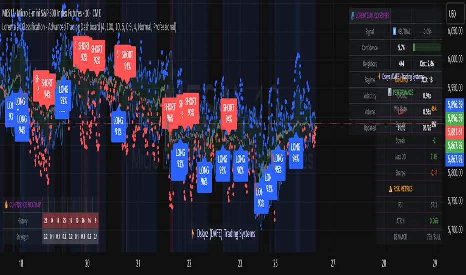
Lorentzian Classification - Advanced Trading DashboardLorentzian Classification - Relativistic Market Analysis
A Journey from Theory to Trading Reality
What began as fascination with Einstein's relativity and Lorentzian geometry has evolved into a practical trading tool that bridges theoretical physics and market dynamics. This indicator represents months of wrestling with complex mathematical concepts, debugging intricate algorithms, and transforming abstract theory into actionable trading signals.
The Theoretical Foundation
Lorentzian Distance in Market Space
Traditional Euclidean distance treats all feature differences equally, but markets don't behave uniformly. Lorentzian distance, borrowed from spacetime geometry, provides a more nuanced similarity measure:
d(x,y) = Σ ln(1 + |xi - yi|)
This logarithmic formulation naturally handles:
Scale invariance: Large price moves don't overwhelm small but significant patterns
Outlier robustness: Extreme values are dampened rather than dominating
Non-linear relationships: Captures market behavior better than linear metrics
K-Nearest Neighbors with Relativistic Weighting
The algorithm searches historical market states for patterns similar to current conditions. Each neighbor receives weight inversely proportional to its Lorentzian distance:
w = 1 / (1 + distance)
This creates a "gravitational" effect where closer patterns have stronger influence on predictions.
The Implementation Challenge
Creating meaningful market features required extensive experimentation:
Price Features: Multi-timeframe momentum (1, 2, 3, 5, 8 bar lookbacks) Volume Features: Relative volume analysis against 20-period average
Volatility Features: ATR and Bollinger Band width normalization Momentum Features: RSI deviation from neutral and MACD/price ratio
Each feature undergoes min-max normalization to ensure equal weighting in distance calculations.
The Prediction Mechanism
For each current market state:
Feature Vector Construction: 12-dimensional representation of market conditions
Historical Search: Scan lookback period for similar patterns using Lorentzian distance
Neighbor Selection: Identify K nearest historical matches
Outcome Analysis: Examine what happened N bars after each match
Weighted Prediction: Combine outcomes using distance-based weights
Confidence Calculation: Measure agreement between neighbors
Technical Hurdles Overcome
Array Management: Complex indexing to prevent look-ahead bias
Distance Calculations: Optimizing nested loops for performance
Memory Constraints: Balancing lookback depth with computational limits
Signal Filtering: Preventing clustering of identical signals
Advanced Dashboard System
Main Control Panel
The primary dashboard provides real-time market intelligence:
Signal Status: Current prediction with confidence percentage
Neighbor Analysis: How many historical patterns match current conditions
Market Regime: Trend strength, volatility, and volume analysis
Temporal Context: Real-time updates with timestamp
Performance Analytics
Comprehensive tracking system monitors:
Win Rate: Percentage of successful predictions
Signal Count: Total predictions generated
Streak Analysis: Current winning/losing sequence
Drawdown Monitoring: Maximum equity decline
Sharpe Approximation: Risk-adjusted performance estimate
Risk Assessment Panel
Multi-dimensional risk analysis:
RSI Positioning: Overbought/oversold conditions
ATR Percentage: Current volatility relative to price
Bollinger Position: Price location within volatility bands
MACD Alignment: Momentum confirmation
Confidence Heatmap
Visual representation of prediction reliability:
Historical Confidence: Last 10 periods of prediction certainty
Strength Analysis: Magnitude of prediction values over time
Pattern Recognition: Color-coded confidence levels for quick assessment
Input Parameters Deep Dive
Core Algorithm Settings
K Nearest Neighbors (1-20): More neighbors create smoother but less responsive signals. Optimal range 5-8 for most markets.
Historical Lookback (50-500): Deeper history improves pattern recognition but reduces adaptability. 100-200 bars optimal for most timeframes.
Feature Window (5-30): Longer windows capture more context but reduce sensitivity. Match to your trading timeframe.
Feature Selection
Price Changes: Essential for momentum and reversal detection Volume Profile: Critical for institutional activity recognition Volatility Measures: Key for regime change detection Momentum Indicators: Vital for trend confirmation
Signal Generation
Prediction Horizon (1-20): How far ahead to predict. Shorter horizons for scalping, longer for swing trading.
Signal Threshold (0.5-0.9): Confidence required for signal generation. Higher values reduce false signals but may miss opportunities.
Smoothing (1-10): EMA applied to raw predictions. More smoothing reduces noise but increases lag.
Visual Design Philosophy
Color Themes
Professional: Corporate blue/red for institutional environments Neon: Cyberpunk cyan/magenta for modern aesthetics
Matrix: Green/red hacker-inspired palette Classic: Traditional trading colors
Information Hierarchy
The dashboard system prioritizes information by importance:
Primary Signals: Largest, most prominent display
Confidence Metrics: Secondary but clearly visible
Supporting Data: Detailed but unobtrusive
Historical Context: Available but not distracting
Trading Applications
Signal Interpretation
Long Signals: Prediction > threshold with high confidence
Look for volume confirmation
- Check trend alignment
- Verify support levels
Short Signals: Prediction < -threshold with high confidence
Confirm with resistance levels
- Check for distribution patterns
- Verify momentum divergence
- Market Regime Adaptation
Trending Markets: Higher confidence in directional signals
Ranging Markets: Focus on reversal signals at extremes
Volatile Markets: Require higher confidence thresholds
Low Volume: Reduce position sizes, increase caution
Risk Management Integration
Confidence-Based Sizing: Larger positions for higher confidence signals
Regime-Aware Stops: Wider stops in volatile regimes
Multi-Timeframe Confirmation: Align signals across timeframes
Volume Confirmation: Require volume support for major signals
Originality and Innovation
This indicator represents genuine innovation in several areas:
Mathematical Approach
First application of Lorentzian geometry to market pattern recognition. Unlike Euclidean-based systems, this naturally handles market non-linearities.
Feature Engineering
Sophisticated multi-dimensional feature space combining price, volume, volatility, and momentum in normalized form.
Visualization System
Professional-grade dashboard system providing comprehensive market intelligence in intuitive format.
Performance Tracking
Real-time performance analytics typically found only in institutional trading systems.
Development Journey
Creating this indicator involved overcoming numerous technical challenges:
Mathematical Complexity: Translating theoretical concepts into practical code
Performance Optimization: Balancing accuracy with computational efficiency
User Interface Design: Making complex data accessible and actionable
Signal Quality: Filtering noise while maintaining responsiveness
The result is a tool that brings institutional-grade analytics to individual traders while maintaining the theoretical rigor of its mathematical foundation.
Best Practices
- Parameter Optimization
- Start with default settings and adjust based on:
Market Characteristics: Volatile vs. stable
Trading Timeframe: Scalping vs. swing trading
Risk Tolerance: Conservative vs. aggressive
Signal Confirmation
Never trade on Lorentzian signals alone:
Price Action: Confirm with support/resistance
Volume: Verify with volume analysis
Multiple Timeframes: Check higher timeframe alignment
Market Context: Consider overall market conditions
Risk Management
Position Sizing: Scale with confidence levels
Stop Losses: Adapt to market volatility
Profit Targets: Based on historical performance
Maximum Risk: Never exceed 2-3% per trade
Disclaimer
This indicator is for educational and research purposes only. It does not constitute financial advice or guarantee profitable trading results. The Lorentzian classification system reveals market patterns but cannot predict future price movements with certainty. Always use proper risk management, conduct your own analysis, and never risk more than you can afford to lose.
Market dynamics are inherently uncertain, and past performance does not guarantee future results. This tool should be used as part of a comprehensive trading strategy, not as a standalone solution.
Bringing the elegance of relativistic geometry to market analysis through sophisticated pattern recognition and intuitive visualization.
Thank you for sharing the idea. You're more than a follower, you're a leader!
@vasanthgautham1221
Trade with precision. Trade with insight.
— Dskyz , for DAFE Trading Systems
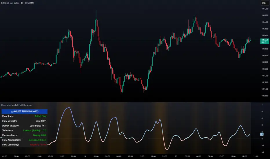
PhenLabs - Market Fluid Dynamics📊 Market Fluid Dynamics -
Version: PineScript™ v6
📌 Description
The Market Fluid Dynamics - Phen indicator is a new thinking regarding market analysis by modeling price action, volume, and volatility using a fluid system. It attempts to offer traders control over more profound market forces, such as momentum (speed), resistance (thickness), and buying/selling pressure. By visualizing such dynamics, the script allows the traders to decide on the prevailing market flow, its power, likely continuations, and zones of calmness and chaos, and thereby allows improved decision-making.
This measure avoids the usual difficulty of reconciling multiple, often contradictory, market indications by including them within a single overarching model. It moves beyond traditional binary indicators by providing a multi-dimensional view of market behavior, employing fluid dynamic analogs to describe complex interactions in an accessible manner.
🚀 Points of Innovation
Integrated Fluid Dynamics Model: Combines velocity, viscosity, pressure, and turbulence into a single indicator.
Normalized Metrics: Uses ATR and other normalization techniques for consistent readings across different assets and timeframes.
Dynamic Flow Visualization: Main flow line changes color and intensity based on direction and strength.
Turbulence Background: Visually represents market stability with a gradient background, from calm to turbulent.
Comprehensive Dashboard: Provides an at-a-glance summary of key fluid dynamic metrics.
Multi-Layer Smoothing: Employs several layers of EMA smoothing for a clearer, more responsive main flow line.
🔧 Core Components
Velocity Component: Measures price momentum (first derivative of price), normalized by ATR. It indicates the speed and direction of price changes.
Viscosity Component: Represents market resistance to price changes, derived from ATR relative to its historical average. Higher viscosity suggests it’s harder for prices to move.
Pressure Component: Quantifies the force created by volume and price range (close - open), normalized by ATR. It reflects buying or selling pressure.
Turbulence Detection: Calculates a Reynolds number equivalent to identify market stability, ranging from laminar (stable) to turbulent (chaotic).
Main Flow Indicator: Combines the above components, applying sensitivity and smoothing, to generate a primary signal of market direction and strength.
🔥 Key Features
Advanced Smoothing Algorithm: Utilizes multiple EMA layers on the raw flow calculation for a fluid and responsive main flow line, reducing noise while maintaining sensitivity.
Gradient Flow Coloring: The main flow line dynamically changes color from light to deep blue for bullish flow and light to deep red for bearish flow, with intensity reflecting flow strength. This provides an immediate visual cue of market sentiment and momentum.
Turbulence Level Background: The chart background changes color based on calculated turbulence (from calm gray to vibrant orange), offering an intuitive understanding of market stability and potential for erratic price action.
Informative Dashboard: A customizable on-screen table displays critical metrics like Flow State, Flow Strength, Market Viscosity, Turbulence, Pressure Force, Flow Acceleration, and Flow Continuity, allowing traders to quickly assess current market conditions.
Configurable Lookback and Sensitivity: Users can adjust the base lookback period for calculations and the sensitivity of the flow to viscosity, tailoring the indicator to different trading styles and market conditions.
Alert Conditions: Pre-defined alerts for flow direction changes (positive/negative crossover of zero line) and detection of high turbulence states.
🎨 Visualization
Main Flow Line: A smoothed line plotted below the main chart, colored blue for bullish flow and red for bearish flow. The intensity of the color (light to dark) indicates the strength of the flow. This line crossing the zero line can signal a change in market direction.
Zero Line: A dotted horizontal line at the zero level, serving as a baseline to gauge whether the market flow is positive (bullish) or negative (bearish).
Turbulence Background: The indicator pane’s background color changes based on the calculated turbulence level. A calm, almost transparent gray indicates low turbulence (laminar flow), while a more vibrant, semi-transparent orange signifies high turbulence. This helps traders visually assess market stability.
Dashboard Table: An optional table displayed on the chart, showing key metrics like ‘Flow State’, ‘Flow Strength’, ‘Market Viscosity’, ‘Turbulence’, ‘Pressure Force’, ‘Flow Acceleration’, and ‘Flow Continuity’ with their current values and qualitative descriptions (e.g., ‘Bullish Flow’, ‘Laminar (Stable)’).
📖 Usage Guidelines
Setting Categories
Show Dashboard - Default: true; Range: true/false; Description: Toggles the visibility of the Market Fluid Dynamics dashboard on the chart. Enable to see key metrics at a glance.
Base Lookback Period - Default: 14; Range: 5 - (no upper limit, practical limits apply); Description: Sets the primary lookback period for core calculations like velocity, ATR, and volume SMA. Shorter periods make the indicator more sensitive to recent price action, while longer periods provide a smoother, slower signal.
Flow Sensitivity - Default: 0.5; Range: 0.1 - 1.0 (step 0.1); Description: Adjusts how much the market viscosity dampens the raw flow. A lower value means viscosity has less impact (flow is more sensitive to raw velocity/pressure), while a higher value means viscosity has a greater dampening effect.
Flow Smoothing - Default: 5; Range: 1 - 20; Description: Controls the length of the EMA smoothing applied to the main flow line. Higher values result in a smoother flow line but with more lag; lower values make it more responsive but potentially noisier.
Dashboard Position - Default: ‘Top Right’; Range: ‘Top Right’, ‘Top Left’, ‘Bottom Right’, ‘Bottom Left’, ‘Middle Right’, ‘Middle Left’; Description: Determines the placement of the dashboard on the chart.
Header Size - Default: ‘Normal’; Range: ‘Tiny’, ‘Small’, ‘Normal’, ‘Large’, ‘Huge’; Description: Sets the text size for the dashboard header.
Values Size - Default: ‘Small’; Range: ‘Tiny’, ‘Small’, ‘Normal’, ‘Large’; Description: Sets the text size for the metric values in the dashboard.
✅ Best Use Cases
Trend Identification: Identifying the dominant market flow (bullish or bearish) and its strength to trade in the direction of the prevailing trend.
Momentum Confirmation: Using the flow strength and acceleration to confirm the conviction behind price movements.
Volatility Assessment: Utilizing the turbulence metric to gauge market stability, helping to adjust position sizing or avoid choppy conditions.
Reversal Spotting: Watching for divergences between price and flow, or crossovers of the main flow line above/below the zero line, as potential reversal signals, especially when combined with changes in pressure or viscosity.
Swing Trading: Leveraging the smoothed flow line to capture medium-term market swings, entering when flow aligns with the desired trade direction and exiting when flow weakens or reverses.
Intraday Scalping: Using shorter lookback periods and higher sensitivity to identify quick shifts in flow and turbulence for short-term trading opportunities, particularly in liquid markets.
⚠️ Limitations
Lagging Nature: Like many indicators based on moving averages and lookback periods, the main flow line can lag behind rapid price changes, potentially leading to delayed signals.
Whipsaws in Ranging Markets: During periods of low volatility or sideways price action (high viscosity, low flow strength), the indicator might produce frequent buy/sell signals (whipsaws) as the flow oscillates around the zero line.
Not a Standalone System: While comprehensive, it should be used in conjunction with other forms of analysis (e.g., price action, support/resistance levels, other indicators) and not as a sole basis for trading decisions.
Subjectivity in Interpretation: While the dashboard provides quantitative values, the interpretation of “strong” flow, “high” turbulence, or “significant” acceleration can still have a subjective element depending on the trader’s strategy and risk tolerance.
💡 What Makes This Unique
Fluid Dynamics Analogy: Its core strength lies in translating complex market interactions into an intuitive fluid dynamics framework, making concepts like momentum, resistance, and pressure easier to visualize and understand.
Market View: Instead of focusing on a single aspect (like just momentum or just volatility), it integrates multiple factors (velocity, viscosity, pressure, turbulence) to provide a more comprehensive picture of market conditions.
Adaptive Visualization: The dynamic coloring of the flow line and the turbulence background provide immediate, adaptive visual feedback that changes with market conditions.
🔬 How It Works
Price Velocity Calculation: The indicator first calculates price velocity by measuring the rate of change of the closing price over a given ‘lookback’ period. The raw velocity is then normalized by the Average True Range (ATR) of the same lookback period. Normalization enables comparison of momentum between assets or timeframes by scaling for volatility. This is the direction and speed of initial price movement.
Viscosity Calculation: Market ‘viscosity’ or resistance to price movement is determined by looking at the current ATR relative to its longer-term average (SMA of ATR over lookback * 2). The further the current ATR is above its average, the lower the viscosity (less resistance to price movement), and vice-versa. The script inverts this relationship and bounds it so that rising viscosity means more resistance.
Pressure Force Measurement: A ‘pressure’ variable is calculated as a function of the ratio of current volume to its simple moving average, multiplied by the price range (close - open) and normalized by ATR. This is designed to measure the force behind price movement created by volume and intraday price thrusts. This pressure is smoothed by an EMA.
Turbulence State Evaluation: A equivalent ‘Reynolds number’ is calculated by dividing the absolute normalized velocity by the viscosity. This is the proclivity of the market to move in a chaotic or orderly fashion. This ‘reynoldsValue’ is smoothed with an EMA to get the ‘turbulenceState’, which indicates if the market is laminar (stable), transitional, or turbulent.
Main Flow Derivation: The ‘rawFlow’ is calculated by taking the normalized velocity, dampening its impact based on the ‘viscosity’ and user-input ‘sensitivity’, and orienting it by the sign of the smoothed ‘pressureSmooth’. The ‘rawFlow’ is then put through multiple layers of exponential moving average (EMA) smoothing (with ‘smoothingLength’ and derived values) to reach the final ‘mainFlow’ line. The extensive smoothing is designed to give a smooth and clear visualization of the overall market direction and magnitude.
Dashboard Metrics Compilation: Additional metrics like flow acceleration (derivative of mainFlow), and flow continuity (correlation between close and volume) are calculated. All primary components (Flow State, Strength, Viscosity, Turbulence, Pressure, Acceleration, Continuity) are then presented in a user-configurable dashboard for ease of monitoring.
💡 Note:
The “Market Fluid Dynamics - Phen” indicator is designed to offer a unique perspective on market behavior by applying principles from fluid dynamics. It’s most effective when used to understand the underlying forces driving price rather than as a direct buy/sell signal generator in isolation. Experiment with the settings, particularly the ‘Base Lookback Period’, ‘Flow Sensitivity’, and ‘Flow Smoothing’, to find what best suits your trading style and the specific asset you are analyzing. Always combine its insights with robust risk management practices.
Machine Learning RSI ║ BullVisionOverview:
Introducing the Machine Learning RSI with KNN Adaptation – a cutting-edge momentum indicator that blends the classic Relative Strength Index (RSI) with machine learning principles. By leveraging K-Nearest Neighbors (KNN), this indicator aims at identifying historical patterns that resemble current market behavior and uses this context to refine RSI readings with enhanced sensitivity and responsiveness.
Unlike traditional RSI models, which treat every market environment the same, this version adapts in real-time based on how similar past conditions evolved, offering an analytical edge without relying on predictive assumptions.
Key Features:
🔁 KNN-Based RSI Refinement
This indicator uses a machine learning algorithm (K-Nearest Neighbors) to compare current RSI and price action characteristics to similar historical conditions. The resulting RSI is weighted accordingly, producing a dynamically adjusted value that reflects historical context.
📈 Multi-Feature Similarity Analysis
Pattern similarity is calculated using up to five customizable features:
RSI level
RSI momentum
Volatility
Linear regression slope
Price momentum
Users can adjust how many features are used to tailor the behavior of the KNN logic.
🧠 Machine Learning Weight Control
The influence of the machine learning model on the final RSI output can be fine-tuned using a simple slider. This lets you blend traditional RSI and machine learning-enhanced RSI to suit your preferred level of adaptation.
🎛️ Adaptive Filtering
Additional smoothing options (Kalman Filter, ALMA, Double EMA) can be applied to the RSI, offering better visual clarity and helping to reduce noise in high-frequency environments.
🎨 Visual & Accessibility Settings
Custom color palettes, including support for color vision deficiencies, ensure that trend coloring remains readable for all users. A built-in neon mode adds high-contrast visuals to improve RSI visibility across dark or light themes.
How It Works:
Similarity Matching with KNN:
At each candle, the current RSI and optional market characteristics are compared to historical bars using a KNN search. The algorithm selects the closest matches and averages their RSI values, weighted by similarity. The more similar the pattern, the greater its influence.
Feature-Based Weighting:
Similarity is determined using normalized values of the selected features, which gives a more refined result than RSI alone. You can choose to use only 1 (RSI) or up to all 5 features for deeper analysis.
Filtering & Blending:
After the machine learning-enhanced RSI is calculated, it can be optionally smoothed using advanced filters to suppress short-term noise or sharp spikes. This makes it easier to evaluate RSI signals in different volatility regimes.
Parameters Explained:
📊 RSI Settings:
Set the base RSI length and select your preferred smoothing method from 10+ moving average types (e.g., EMA, ALMA, TEMA).
🧠 Machine Learning Controls:
Enable or disable the KNN engine
Select how many nearest neighbors to compare (K)
Choose the number of features used in similarity detection
Control how much the machine learning engine affects the RSI calculation
🔍 Filtering Options:
Enable one of several advanced smoothing techniques (Kalman Filter, ALMA, Double EMA) to adjust the indicator’s reactivity and stability.
📏 Threshold Levels:
Define static overbought/oversold boundaries or reference dynamically adjusted thresholds based on historical context identified by the KNN algorithm.
🎨 Visual Enhancements:
Select between trend-following or impulse coloring styles. Customize color palettes to accommodate different types of color blindness. Enable neon-style effects for visual clarity.
Use Cases:
Swing & Trend Traders
Can use the indicator to explore how current RSI readings compare to similar market phases, helping to assess trend strength or potential turning points.
Intraday Traders
Benefit from adjustable filters and fast-reacting smoothing to reduce noise in shorter timeframes while retaining contextual relevance.
Discretionary Analysts
Use the adaptive OB/OS thresholds and visual cues to supplement broader confluence zones or market structure analysis.
Customization Tips:
Higher Volatility Periods: Use more neighbors and enable filtering to reduce noise.
Lower Volatility Markets: Use fewer features and disable filtering for quicker RSI adaptation.
Deeper Contextual Analysis: Increase KNN lookback and raise the feature count to refine pattern recognition.
Accessibility Needs: Switch to Deuteranopia or Monochrome mode for clearer visuals in specific color vision conditions.
Final Thoughts:
The Machine Learning RSI combines familiar momentum logic with statistical context derived from historical similarity analysis. It does not attempt to predict price action but rather contextualizes RSI behavior with added nuance. This makes it a valuable tool for those looking to elevate traditional RSI workflows with adaptive, research-driven enhancements.

Wall Street Ai**Wall Street Ai – Advanced Technical Indicator for Market Analysis**
**Overview**
Wall Street Ai is an advanced, AI-powered technical indicator meticulously engineered to provide traders with in-depth market analysis and insight. By leveraging state-of-the-art artificial intelligence algorithms and comprehensive historical price data, Wall Street Ai is designed to identify significant market turning points and key price levels. Its sophisticated analytical framework enables traders to uncover potential shifts in market momentum, assisting in the formulation of strategic trading decisions while maintaining the highest standards of objectivity and reliability.
**Key Features**
- **Intelligent Pattern Recognition:**
Wall Street Ai employs advanced machine learning techniques to analyze historical price movements and detect recurring patterns. This capability allows it to differentiate between typical market noise and meaningful signals indicative of potential trend reversals.
- **Robust Noise Reduction:**
The indicator incorporates a refined volatility filtering system that minimizes the impact of minor price fluctuations. By isolating significant price movements, it ensures that the analytical output focuses on substantial market shifts rather than ephemeral variations.
- **Customizable Analytical Parameters:**
With a wide range of adjustable settings, Wall Street Ai can be fine-tuned to align with diverse trading strategies and risk appetites. Traders can modify sensitivity, threshold levels, and other critical parameters to optimize the indicator’s performance under various market conditions.
- **Comprehensive Data Analysis:**
By harnessing the power of artificial intelligence, Wall Street Ai performs a deep analysis of historical data, identifying statistically significant highs and lows. This analysis not only reflects past market behavior but also provides valuable insights into potential future turning points, thereby enhancing the predictive aspect of your trading strategy.
- **Adaptive Market Insights:**
The indicator’s dynamic algorithm continuously adjusts to current market conditions, adapting its analysis based on real-time data inputs. This adaptive quality ensures that the indicator remains relevant and effective across different market environments, whether the market is trending strongly, consolidating, or experiencing volatility.
- **Objective and Reliable Analysis:**
Wall Street Ai is built on a foundation of robust statistical methods and rigorous data validation. Its outputs are designed to be objective and free from any exaggerated claims, ensuring that traders receive a clear, unbiased view of market conditions.
**How It Works**
Wall Street Ai integrates advanced AI and deep learning methodologies to analyze a vast array of historical price data. Its core algorithm identifies and evaluates critical market levels by detecting patterns that have historically preceded significant market movements. By filtering out non-essential fluctuations, the indicator emphasizes key price extremes and trend changes that are likely to impact market behavior. The system’s adaptive nature allows it to recalibrate its analytical parameters in response to evolving market dynamics, providing a consistently reliable framework for market analysis.
**Usage Recommendations**
- **Optimal Timeframes:**
For the most effective application, it is recommended to utilize Wall Street Ai on higher timeframe charts, such as hourly (H1) or higher. This approach enhances the clarity of the detected patterns and provides a more comprehensive view of long-term market trends.
- **Market Versatility:**
Wall Street Ai is versatile and can be applied across a broad range of financial markets, including Forex, indices, commodities, cryptocurrencies, and equities. Its adaptable design ensures consistent performance regardless of the asset class being analyzed.
- **Complementary Analytical Tools:**
While Wall Street Ai provides profound insights into market behavior, it is best utilized in combination with other analytical tools and techniques. Integrating its analysis with additional indicators—such as trend lines, support/resistance levels, or momentum oscillators—can further refine your trading strategy and enhance decision-making.
- **Strategy Testing and Optimization:**
Traders are encouraged to test Wall Street Ai extensively in a simulated trading environment before deploying it in live markets. This allows for thorough calibration of its settings according to individual trading styles and risk management strategies, ensuring optimal performance across diverse market conditions.
**Risk Management and Best Practices**
Wall Street Ai is intended to serve as an analytical tool that supports informed trading decisions. However, as with any technical indicator, its outputs should be interpreted as part of a comprehensive trading strategy that includes robust risk management practices. Traders should continuously validate the indicator’s findings with additional analysis and maintain a disciplined approach to position sizing and risk control. Regular review and adjustment of trading strategies in response to market changes are essential to mitigate potential losses.
**Conclusion**
Wall Street Ai offers a cutting-edge, AI-driven approach to technical analysis, empowering traders with detailed market insights and the ability to identify potential turning points with precision. Its intelligent pattern recognition, adaptive analytical capabilities, and extensive noise reduction make it a valuable asset for both experienced traders and those new to market analysis. By integrating Wall Street Ai into your trading toolkit, you can enhance your understanding of market dynamics and develop a more robust, data-driven trading strategy—all while adhering to the highest standards of analytical integrity and performance.

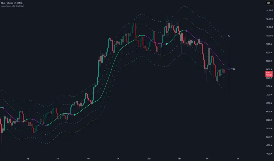
Lowess Channel + (RSI) [ChartPrime]The Lowess Channel + (RSI) indicator applies the LOWESS (Locally Weighted Scatterplot Smoothing) algorithm to filter price fluctuations and construct a dynamic channel. LOWESS is a non-parametric regression method that smooths noisy data by fitting weighted linear regressions at localized segments. This technique is widely used in statistical analysis to reveal trends while preserving data structure.
In this indicator, the LOWESS algorithm is used to create a central trend line and deviation-based bands. The midline changes color based on trend direction, and diamonds are plotted when a trend shift occurs. Additionally, an RSI gauge is positioned at the end of the channel to display the current RSI level in relation to the price bands.
lowess_smooth(src, length, bandwidth) =>
sum_weights = 0.0
sum_weighted_y = 0.0
sum_weighted_xy = 0.0
sum_weighted_x2 = 0.0
sum_weighted_x = 0.0
for i = 0 to length - 1
x = float(i)
weight = math.exp(-0.5 * (x / bandwidth) * (x / bandwidth))
y = nz(src , 0)
sum_weights := sum_weights + weight
sum_weighted_x := sum_weighted_x + weight * x
sum_weighted_y := sum_weighted_y + weight * y
sum_weighted_xy := sum_weighted_xy + weight * x * y
sum_weighted_x2 := sum_weighted_x2 + weight * x * x
mean_x = sum_weighted_x / sum_weights
mean_y = sum_weighted_y / sum_weights
beta = (sum_weighted_xy - mean_x * mean_y * sum_weights) / (sum_weighted_x2 - mean_x * mean_x * sum_weights)
alpha = mean_y - beta * mean_x
alpha + beta * float(length / 2) // Centered smoothing
⯁ KEY FEATURES
LOWESS Price Filtering – Smooths price fluctuations to reveal the underlying trend with minimal lag.
Dynamic Trend Coloring – The midline changes color based on trend direction (e.g., bullish or bearish).
Trend Shift Diamonds – Marks points where the midline color changes, indicating a possible trend shift.
Deviation-Based Bands – Expands above and below the midline using ATR-based multipliers for volatility tracking.
RSI Gauge Display – A vertical gauge at the right side of the chart shows the current RSI level relative to the price channel.
Fully Customizable – Users can adjust LOWESS length, band width, colors, and enable or disable the RSI gauge and adjust RSIlength.
⯁ HOW TO USE
Use the LOWESS midline as a trend filter —bullish when green, bearish when purple.
Watch for trend shift diamonds as potential entry or exit signals.
Utilize the price bands to gauge overbought and oversold zones based on volatility.
Monitor the RSI gauge to confirm trend strength—high RSI near upper bands suggests overbought conditions, while low RSI near lower bands indicates oversold conditions.
⯁ CONCLUSION
The Lowess Channel + (RSI) indicator offers a powerful way to analyze market trends by applying a statistically robust smoothing algorithm. Unlike traditional moving averages, LOWESS filtering provides a flexible, responsive trendline that adapts to price movements. The integrated RSI gauge enhances decision-making by displaying momentum conditions alongside trend dynamics. Whether used for trend-following or mean reversion strategies, this indicator provides traders with a well-rounded perspective on market behavior.
*Auto Backtest & Optimize EngineFull-featured Engine for Automatic Backtesting and parameter optimization. Allows you to test millions of different combinations of stop-loss and take profit parameters, including on any connected indicators.
⭕️ Key Futures
Quickly identify the optimal parameters for your strategy.
Automatically generate and test thousands of parameter combinations.
A simple Genetic Algorithm for result selection.
Saves time on manual testing of multiple parameters.
Detailed analysis, sorting, filtering and statistics of results.
Detailed control panel with many tooltips.
Display of key metrics: Profit, Win Rate, etc..
Comprehensive Strategy Score calculation.
In-depth analysis of the performance of different types of stop-losses.
Possibility to use to calculate the best Stop-Take parameters for your position.
Ability to test your own functions and signals.
Customizable visualization of results.
Flexible Stop-Loss Settings:
• Auto ━ Allows you to test all types of Stop Losses at once(listed below).
• S.VOLATY ━ Static stop based on volatility (Fixed, ATR, STDEV).
• Trailing ━ Classic trailing stop following the price.
• Fast Trail ━ Accelerated trailing stop that reacts faster to price movements.
• Volatility ━ Dynamic stop based on volatility indicators.
• Chandelier ━ Stop based on price extremes.
• Activator ━ Dynamic stop based on SAR.
• MA ━ Stop based on moving averages (9 different types).
• SAR ━ Parabolic SAR (Stop and Reverse).
Advanced Take-Profit Options:
• R:R: Risk/Reward ━ sets TP based on SL size.
• T.VOLATY ━ Calculation based on volatility indicators (Fixed, ATR, STDEV).
Testing Modes:
• Stops ━ Cyclical stop-loss testing
• Pivot Point Example ━ Example of using pivot points
• External Example ━ Built-in example how test functions with different parameters
• External Signal ━ Using external signals
⭕️ Usage
━ First Steps:
When opening, select any point on the chart. It will not affect anything until you turn on Manual Start mode (more on this below).
The chart will immediately show the best results of the default Auto mode. You can switch Part's to try to find even better results in the table.
Now you can display any result from the table on the chart by entering its ID in the settings.
Repeat steps 3-4 until you determine which type of Stop Loss you like best. Then set it in the settings instead of Auto mode.
* Example: I flipped through 14 parts before I liked the first result and entered its ID so I could visually evaluate it on the chart.
Then select the stop loss type, choose it in place of Auto mode and repeat steps 3-4 or immediately follow the recommendations of the algorithm.
Now the Genetic Algorithm at the bottom right will prompt you to enter the Parameters you need to search for and select even better results.
Parameters must be entered All at once before they are updated. Enter recommendations strictly in fields with the same names.
Repeat steps 5-6 until there are approximately 10 Part's left or as you like. And after that, easily pour through the remaining Parts and select the best parameters.
━ Example of the finished result.
━ Example of use with Takes
You can also test at the same time along with Take Profit. In this example, I simply enabled Risk/Reward mode and immediately specified in the TP field Maximum RR, Minimum RR and Step. So in this example I can test (3-1) / 0.1 = 20 Takes of different sizes. There are additional tips in the settings.
━
* Soon you will start to understand how the system works and things will become much easier.
* If something doesn't work, just reset the engine settings and start over again.
* Use the tips I have left in the settings and on the Panel.
━ Details:
Sort ━ Sorting results by Score, Profit, Trades, etc..
Filter ━ Filtring results by Score, Profit, Trades, etc..
Trade Type ━ Ability to disable Long\Short but only from statistics.
BackWin ━ Backtest Window Number of Candle the script can test.
Manual Start ━ Enabling it will allow you to call a Stop from a selected point. which you selected when you started the engine.
* If you have a real open position then this mode can help to save good Stop\Take for it.
1 - 9 Сheckboxs ━ Allow you to disable any stop from Auto mode.
Ex Source - Allow you to test Stops/Takes from connected indicators.
Connection guide:
//@version=6
indicator("My script")
rsi = ta.rsi(close, 14)
buy = not na(rsi) and ta.crossover (rsi, 40) // OS = 40
sell = not na(rsi) and ta.crossunder(rsi, 60) // OB = 60
Signal = buy ? +1 : sell ? -1 : 0
plot(Signal, "🔌Connector🔌", display = display.none)
* Format the signal for your indicator in a similar style and then select it in Ex Source.
⭕️ How it Works
Hypothesis of Uniform Distribution of Rare Elements After Mixing.
'This hypothesis states that if an array of N elements contains K valid elements, then after mixing, these valid elements will be approximately uniformly distributed.'
'This means that in a random sample of k elements, the proportion of valid elements should closely match their proportion in the original array, with some random variation.'
'According to the central limit theorem, repeated sampling will result in an average count of valid elements following a normal distribution.'
'This supports the assumption that the valid elements are evenly spread across the array.'
'To test this hypothesis, we can conduct an experiment:'
'Create an array of 1,000,000 elements.'
'Select 1,000 random elements (1%) for validation.'
'Shuffle the array and divide it into groups of 1,000 elements.'
'If the hypothesis holds, each group should contain, on average, 1~ valid element, with minor variations.'
* I'd like to attach more details to My hypothesis but it won't be very relevant here. Since this is a whole separate topic, I will leave the minimum part for understanding the engine.
Practical Application
To apply this hypothesis, I needed a way to generate and thoroughly mix numerous possible combinations. Within Pine, generating over 100,000 combinations presents significant challenges, and storing millions of combinations requires excessive resources.
I developed an efficient mechanism that generates combinations in random order to address these limitations. While conventional methods often produce duplicates or require generating a complete list first, my approach guarantees that the first 10% of possible combinations are both unique and well-distributed. Based on my hypothesis, this sampling is sufficient to determine optimal testing parameters.
Most generators and randomizers fail to accommodate both my hypothesis and Pine's constraints. My solution utilizes a simple Linear Congruential Generator (LCG) for pseudo-randomization, enhanced with prime numbers to increase entropy during generation. I pre-generate the entire parameter range and then apply systematic mixing. This approach, combined with a hybrid combinatorial array-filling technique with linear distribution, delivers excellent generation quality.
My engine can efficiently generate and verify 300 unique combinations per batch. Based on the above, to determine optimal values, only 10-20 Parts need to be manually scrolled through to find the appropriate value or range, eliminating the need for exhaustive testing of millions of parameter combinations.
For the Score statistic I applied all the same, generated a range of Weights, distributed them randomly for each type of statistic to avoid manual distribution.
Score ━ based on Trade, Profit, WinRate, Profit Factor, Drawdown, Sharpe & Sortino & Omega & Calmar Ratio.
⭕️ Notes
For attentive users, a little tricks :)
To save time, switch parts every 3 seconds without waiting for it to load. After 10-20 parts, stop and wait for loading. If the pause is correct, you can switch between the rest of the parts without loading, as they will be cached. This used to work without having to wait for a pause, but now it does slower. This will save a lot of time if you are going to do a deeper backtest.
Sometimes you'll get the error “The scripts take too long to execute.”
For a quick fix you just need to switch the TF or Ticker back and forth and most likely everything will load.
The error appears because of problems on the side of the site because the engine is very heavy. It can also appear if you set too long a period for testing in BackWin or use a heavy indicator for testing.
Manual Start - Allow you to Start you Result from any point. Which in turn can help you choose a good stop-stick for your real position.
* It took me half a year from idea to current realization. This seems to be one of the few ways to build something automatic in backtest format and in this particular Pine environment. There are already better projects in other languages, and they are created much easier and faster because there are no limitations except for personal PC. If you see solutions to improve this system I would be glad if you share the code. At the moment I am tired and will continue him not soon.
Also You can use my previosly big Backtest project with more manual settings(updated soon)

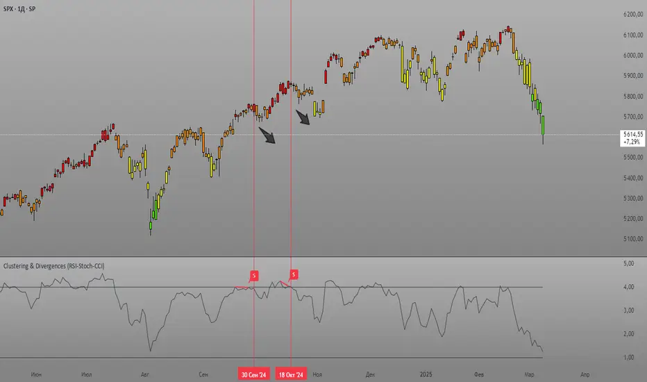
Clustering & Divergences (RSI-Stoch-CCI) [Sam SDF-Solutions]The Clustering & Divergences (RSI-Stoch-CCI) indicator is a comprehensive technical analysis tool that consolidates three popular oscillators—Relative Strength Index (RSI), Stochastic, and Commodity Channel Index (CCI)—into one unified metric called the Score. This Score offers traders an aggregated view of market conditions, allowing them to quickly identify whether the market is oversold, balanced, or overbought.
Functionality:
Oscillator Clustering: The indicator calculates the values of RSI, Stochastic, and CCI using user-defined periods. These oscillator values are then normalized using one of three available methods: MinMax, Z-Score, or Z-Bins.
Score Calculation: Each normalized oscillator value is multiplied by its respective weight (which the user can adjust), and the weighted values are summed to generate an overall Score. This Score serves as a single, interpretable metric representing the combined oscillator behavior.
Market Clustering: The indicator performs clustering on the Score over a configurable window. By dividing the Score range into a set number of clusters (also configurable), the tool visually represents the market’s state. Each cluster is assigned a unique color so that traders can quickly see if the market is trending toward oversold, balanced, or overbought conditions.
Divergence Detection: The script automatically identifies both Regular and Hidden divergences between the price action and the Score. By using pivot detection on both price and Score data, the indicator marks potential reversal signals on the chart with labels and connecting lines. This helps in pinpointing moments when the price and the underlying oscillator dynamics diverge.
Customization Options: Users have full control over the indicator’s behavior. They can adjust:
The periods for each oscillator (RSI, Stochastic, CCI).
The weights applied to each oscillator in the Score calculation.
The normalization method and its manual boundaries.
The number of clusters and whether to invert the cluster order.
Parameters for divergence detection (such as pivot sensitivity and the minimum/maximum bar distance between pivots).
Visual Enhancements:
Depending on the user’s preference, either the Score or the Cluster Index (derived from the clustering process) is plotted on the chart. Additionally, the script changes the color of the price bars based on the identified cluster, providing an at-a-glance visual cue of the current market regime.
Logic & Methodology:
Input Parameters: The script starts by accepting user inputs for clustering settings, oscillator periods, weights, divergence detection, and manual boundary definitions for normalization.
Oscillator Calculation & Normalization: It computes RSI, Stochastic, and CCI values from the price data. These values are then normalized using either the MinMax method (scaling between a lower and upper band) or the Z-Score method (standardizing based on mean and standard deviation), or using Z-Bins for an alternative scaling approach.
Score Computation: Each normalized oscillator is multiplied by its corresponding weight. The sum of these products results in the overall Score that represents the combined oscillator behavior.
Clustering Algorithm: The Score is evaluated over a moving window to determine its minimum and maximum values. Using these values, the script calculates a cluster index that divides the Score into a predefined number of clusters. An option to invert the cluster calculation is provided to adjust the interpretation of the clustering.
Divergence Analysis: The indicator employs pivot detection (using left and right bar parameters) on both the price and the Score. It then compares recent pivot values to detect regular and hidden divergences. When a divergence is found, the script plots labels and optional connecting lines to highlight these key moments on the chart.
Plotting: Finally, based on the user’s selection, the indicator plots either the Score or the Cluster Index. It also overlays manual boundary lines (for the chosen normalization method) and adjusts the bar colors according to the cluster to provide clear visual feedback on market conditions.
_________
By integrating multiple oscillator signals into one cohesive tool, the Clustering & Divergences (RSI-Stoch-CCI) indicator helps traders minimize subjective analysis. Its dynamic clustering and automated divergence detection provide a streamlined method for assessing market conditions and potentially enhancing the accuracy of trading decisions.
For further details on using this indicator, please refer to the guide available at:
Percentage Based ZigZag█ OVERVIEW
The Percentage-Based ZigZag indicator is a custom technical analysis tool designed to highlight significant price reversals while filtering out market noise. Unlike many standard zigzag tools that rely solely on fixed price moves or generic trend-following methods, this indicator uses a configurable percentage threshold to dynamically determine meaningful pivot points. This approach not only adapts to different market conditions but also helps traders distinguish between minor fluctuations and truly significant trend shifts—whether scalping on shorter timeframes or analyzing longer-term trends.
█ KEY FEATURES & ORIGINALITY
Dynamic Pivot Detection
The indicator identifies pivot points by measuring the percentage change from the previous extreme (high or low). Only when this change exceeds a user-defined threshold is a new pivot recognized. This method ensures that only substantial moves are considered, making the indicator robust in volatile or noisy markets.
Enhanced ZigZag Visualization
By connecting significant highs and lows with a continuous line, the indicator creates a clear visual map of price swings. Each pivot point is labelled with the corresponding price and the percentage change from the previous pivot, providing immediate quantitative insight into the magnitude of the move.
Trend Reversal Projections
In addition to marking completed reversals, the script computes and displays potential future reversal points based on the current trend’s momentum. This forecasting element gives traders an advanced look at possible turning points, which can be particularly useful for short-term scalping strategies.
Customizable Visual Settings
Users can tailor the appearance by:
• Setting the percentage threshold to control sensitivity.
• Customizing colors for bullish (e.g., green) and bearish (e.g., red) reversals.
• Enabling optional background color changes that visually indicate the prevailing trend.
█ UNDERLYING METHODOLOGY & CALCULATIONS
Percentage-Based Filtering
The script continuously monitors price action and calculates the relative percentage change from the last identified pivot. A new pivot is confirmed only when the price moves a preset percentage away from this pivot, ensuring that minor fluctuations do not trigger false signals.
Pivot Point Logic
The indicator tracks the highest high and the lowest low since the last pivot. When the price reverses by the required percentage from these extremes, the algorithm:
1 — Labels the point as a significant high or low.
2 — Draws a connecting line from the previous pivot to the current one.
3 — Resets the extreme-tracking for detecting the next move.
Real-Time Reversal Estimation
Building on traditional zigzag methods, the script incorporates a projection calculation. By analyzing the current trend’s strength and recent percentage moves, it estimates where a future reversal might occur, offering traders actionable foresight.
█ HOW TO USE THE INDICATOR
1 — Apply the Indicator
• Add the Percentage-Based ZigZag indicator to your trading chart.
2 — Adjust Settings for Your Market
• Percentage Move – Set a threshold that matches your trading style:
- Lower values for sensitive, high-frequency analysis (ideal for scalping).
- Higher values for filtering out noise on longer timeframes.
• Visual Customization – Choose your preferred colors for bullish and bearish signals and enable background color changes for visual trend cues.
• Reversal Projection – Enable or disable the projection feature to display potential upcoming reversal points.
3 — Interpret the Signals
• ZigZag Lines – White lines trace significant high-to-low or low-to-high movements, visually connecting key swing points.
• Pivot Labels – Each pivot is annotated with the exact price level and percentage change, providing quantitative insight into market momentum.
• Trend Projections – When enabled, projected reversal levels offer insight into where the current trend might change.
4 — Integrate with Your Trading Strategy
• Use the indicator to identify support and resistance zones derived from significant pivots.
• Combine the quantitative data (percentage changes) with your risk management strategy to set optimal stop-loss and take-profit levels.
• Experiment with different threshold settings to adapt the indicator for various instruments or market conditions.
█ CONCLUSION
The Percentage-Based ZigZag indicator goes beyond traditional trend-following tools by filtering out market noise and providing clear, quantifiable insights into price action. With its percentage threshold for pivot detection and real-time reversal projections, this original methodology and customizable feature set offer traders a versatile edge for making informed trading decisions.

Cluster Reversal Zones📌 Cluster Reversal Zones – Smart Market Turning Point Detector
📌 Category : Public (Restricted/Closed-Source) Indicator
📌 Designed for : Traders looking for high-accuracy reversal zones based on price clustering & liquidity shifts.
🔍 Overview
The Cluster Reversal Zones Indicator is an advanced market reversal detection tool that helps traders identify key turning points using a combination of price clustering, order flow analysis, and liquidity tracking. Instead of relying on static support and resistance levels, this tool dynamically adjusts to live market conditions, ensuring traders get the most accurate reversal signals possible.
📊 Core Features:
✅ Real-Time Reversal Zone Mapping – Detects high-probability market turning points using price clustering & order flow imbalance.
✅ Liquidity-Based Support/Resistance Detection – Identifies strong rejection zones based on real-time liquidity shifts.
✅ Order Flow Sensitivity for Smart Filtering – Filters out weak reversals by detecting real market participation behind price movements.
✅ Momentum Divergence for Confirmation – Aligns reversal zones with momentum divergences to increase accuracy.
✅ Adaptive Risk Management System – Adjusts risk parameters dynamically based on volatility and trend state.
🔒 Justification for Mashup
The Cluster Reversal Zones Indicator contains custom-built methodologies that extend beyond traditional support/resistance indicators:
✔ Smart Price Clustering Algorithm: Instead of plotting fixed support/resistance lines, this system analyzes historical price clustering to detect active reversal areas.
✔ Order Flow Delta & Liquidity Shift Sensitivity: The tool tracks real-time order flow data, identifying price zones with the highest accumulation or distribution levels.
✔ Momentum-Based Reversal Validation: Unlike traditional indicators, this tool requires a momentum shift confirmation before validating a potential reversal.
✔ Adaptive Reversal Filtering Mechanism: Uses a combination of historical confluence detection + live market validation to improve accuracy.
🛠️ How to Use:
• Works well for reversal traders, scalpers, and swing traders seeking precise turning points.
• Best combined with VWAP, Market Profile, and Delta Volume indicators for confirmation.
• Suitable for Forex, Indices, Commodities, Crypto, and Stock markets.
🚨 Important Note:
For educational & analytical purposes only.
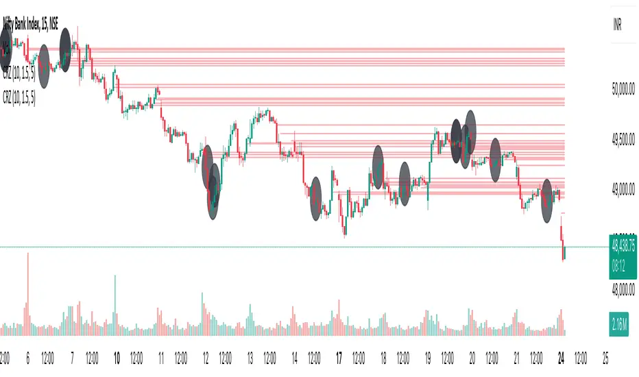
Ehlers Maclaurin Ultimate Smoother [CT]Ehlers Maclaurin Ultimate Smoother
Introduction
The Ehlers Maclaurin Ultimate Smoother is an innovative enhancement of the classic Ehlers SuperSmoother. By leveraging advanced Maclaurin series approximations, this indicator offers superior market analysis and signal generation.
The indicator combines Ehlers' Ultimate Smoother with Maclaurin series approximations to create a more efficient and accurate smoothing mechanism:
Input price data passes through the initial smoothing phase
Maclaurin series approximates trigonometric functions
Enhanced high-pass filter removes market noise
Final smoothing phase produces the output signal
Why the Maclaurin Approach?
The Maclaurin series is a special form of the Taylor series, centered around 0. It provides an efficient way to approximate complex functions using polynomial terms. In this indicator, we use the Maclaurin approach to improve the sine and cosine functions, resulting in:
Faster Calculations: By using polynomial approximations, we significantly reduce computational complexity.
Improved Stability: The approximation provides a more stable numerical basis for calculations.
Preservation of Precision: Despite the approximation, we maintain the precision needed for price smoothing.
Calculations
The indicator employs several key mathematical components:
Maclaurin Series Approximation:
sin(x) ≈ x - x³/3! + x⁵/5! - x⁷/7! + x⁹/9!
cos(x) ≈ 1 - x²/2! + x⁴/4! - x⁶/6! + x⁸/8!
Smoothing Algorithm:
Uses exponential smoothing with optimized coefficients
Implements high-pass filtering for noise reduction
Applies dynamic weighting based on market conditions
Mathematical Foundation
Utilizes Maclaurin series for trigonometric approximation
Implements Ehlers' smoothing principles
Incorporates advanced filtering techniques
Technical Advantages
Signal Processing:
Lag Reduction: Faster signal detection with less delay.
Noise Filtration: Effective elimination of high-frequency noise.
Precision Enhancement: Preservation of critical price movements.
Adaptive Processing: Dynamic response to market volatility.
Visual Enhancements:
Smart color intensity mapping.
Real-time visualization of trend strength.
Adaptive opacity based on movement significance.
Implementation
Core Configuration:
Plot Type: Choose between the original and the Maclaurin enhanced version.
Length: Default set to 30, optimal for daily timeframes.
hpLength: Default set to 10 for enhanced noise reduction.
Advanced Parameters:
The indicator offers advanced control with:
Dual processing modes (Original/Maclaurin).
Dynamic color intensity system.
Customizable smoothing parameters.
Professional Analysis Tools:
Accurate trend reversal identification.
Advanced support/resistance detection.
Superior performance in volatile markets.
Technical Specifications
Maclaurin Series Implementation:
The indicator employs a 5-term Maclaurin series approximation for both sine and cosine, ensuring efficient and accurate computation.
Performance Metrics
Improved processing efficiency.
Reduced memory utilization.
Increased signal accuracy.
Licensing & Attribution
© 2024 Mupsje aka CasaTropical
Professional Credits
Original Ultimate and SuperSmoother concept: John F. Ehlers
Maclaurin enhancement: Casa Tropical (CT)
www.mathsisfun.com

True Amplitude Envelopes (TAE)The True Envelopes indicator is an adaptation of the True Amplitude Envelope (TAE) method, based on the research paper " Improved Estimation of the Amplitude Envelope of Time Domain Signals Using True Envelope Cepstral Smoothing " by Caetano and Rodet. This indicator aims to create an asymmetric price envelope with strong predictive power, closely following the methodology outlined in the paper.
Due to the inherent limitations of Pine Script, the indicator utilizes a Kernel Density Estimator (KDE) in place of the original Cepstral Smoothing technique described in the paper. While this approach was chosen out of necessity rather than superiority, the resulting method is designed to be as effective as possible within the constraints of the Pine environment.
This indicator is ideal for traders seeking an advanced tool to analyze price dynamics, offering insights into potential price movements while working within the practical constraints of Pine Script. Whether used in dynamic mode or with a static setting, the True Envelopes indicator helps in identifying key support and resistance levels, making it a valuable asset in any trading strategy.
Key Features:
Dynamic Mode: The indicator dynamically estimates the fundamental frequency of the price, optimizing the envelope generation process in real-time to capture critical price movements.
High-Pass Filtering: Uses a high-pass filtered signal to identify and smoothly interpolate price peaks, ensuring that the envelope accurately reflects significant price changes.
Kernel Density Estimation: Although implemented as a workaround, the KDE technique allows for flexible and adaptive smoothing of the envelope, aimed at achieving results comparable to the more sophisticated methods described in the original research.
Symmetric and Asymmetric Envelopes: Provides options to select between symmetric and asymmetric envelopes, accommodating various trading strategies and market conditions.
Smoothness Control: Features adjustable smoothness settings, enabling users to balance between responsiveness and the overall smoothness of the envelopes.
The True Envelopes indicator comes with a variety of input settings that allow traders to customize the behavior of the envelopes to match their specific trading needs and market conditions. Understanding each of these settings is crucial for optimizing the indicator's performance.
Main Settings
Source: This is the data series on which the indicator is applied, typically the closing price (close). You can select other price data like open, high, low, or a custom series to base the envelope calculations.
History: This setting determines how much historical data the indicator should consider when calculating the envelopes. A value of 0 will make the indicator process all available data, while a higher value restricts it to the most recent n bars. This can be useful for reducing the computational load or focusing the analysis on recent market behavior.
Iterations: This parameter controls the number of iterations used in the envelope generation algorithm. More iterations will typically result in a smoother envelope, but can also increase computation time. The optimal number of iterations depends on the desired balance between smoothness and responsiveness.
Kernel Style: The smoothing kernel used in the Kernel Density Estimator (KDE). Available options include Sinc, Gaussian, Epanechnikov, Logistic, and Triangular. Each kernel has different properties, affecting how the smoothing is applied. For example, Gaussian provides a smooth, bell-shaped curve, while Epanechnikov is more efficient computationally with a parabolic shape.
Envelope Style: This setting determines whether the envelope should be Static or Dynamic. The Static mode applies a fixed period for the envelope, while the Dynamic mode automatically adjusts the period based on the fundamental frequency of the price data. Dynamic mode is typically more responsive to changing market conditions.
High Q: This option controls the quality factor (Q) of the high-pass filter. Enabling this will increase the Q factor, leading to a sharper cutoff and more precise isolation of high-frequency components, which can help in better identifying significant price peaks.
Symmetric: This setting allows you to choose between symmetric and asymmetric envelopes. Symmetric envelopes maintain an equal distance from the central price line on both sides, while asymmetric envelopes can adjust differently above and below the price line, which might better capture market conditions where upside and downside volatility are not equal.
Smooth Envelopes: When enabled, this setting applies additional smoothing to the envelopes. While this can reduce noise and make the envelopes more visually appealing, it may also decrease their responsiveness to sudden market changes.
Dynamic Settings
Extra Detrend: This setting toggles an additional high-pass filter that can be applied when using a long filter period. The purpose is to further detrend the data, ensuring that the envelope focuses solely on the most recent price oscillations.
Filter Period Multiplier: This multiplier adjusts the period of the high-pass filter dynamically based on the detected fundamental frequency. Increasing this multiplier will lengthen the period, making the filter less sensitive to short-term price fluctuations.
Filter Period (Min) and Filter Period (Max): These settings define the minimum and maximum bounds for the high-pass filter period. They ensure that the filter period stays within a reasonable range, preventing it from becoming too short (and overly sensitive) or too long (and too sluggish).
Envelope Period Multiplier: Similar to the filter period multiplier, this adjusts the period for the envelope generation. It scales the period dynamically to match the detected price cycles, allowing for more precise envelope adjustments.
Envelope Period (Min) and Envelope Period (Max): These settings establish the minimum and maximum bounds for the envelope period, ensuring the envelopes remain adaptive without becoming too reactive or too slow.
Static Settings
Filter Period: In static mode, this setting determines the fixed period for the high-pass filter. A shorter period will make the filter more responsive to price changes, while a longer period will smooth out more of the price data.
Envelope Period: This setting specifies the fixed period used for generating the envelopes in static mode. It directly influences how tightly or loosely the envelopes follow the price action.
TAE Smoothing: This controls the degree of smoothing applied during the TAE process in static mode. Higher smoothing values result in more gradual envelope curves, which can be useful in reducing noise but may also delay the envelope’s response to rapid price movements.
Visual Settings
Top Band Color: This setting allows you to choose the color for the upper band of the envelope. This band represents the resistance level in the price action.
Bottom Band Color: Similar to the top band color, this setting controls the color of the lower band, which represents the support level.
Center Line Color: This is the color of the central price line, often referred to as the carrier. It represents the detrended price around which the envelopes are constructed.
Line Width: This determines the thickness of the plotted lines for the top band, bottom band, and center line. Thicker lines can make the envelopes more visible, especially when overlaid on price data.
Fill Alpha: This controls the transparency level of the shaded area between the top and bottom bands. A lower alpha value will make the fill more transparent, while a higher value will make it more opaque, helping to highlight the envelope more clearly.
The envelopes generated by the True Envelopes indicator are designed to provide a more precise and responsive representation of price action compared to traditional methods like Bollinger Bands or Keltner Channels. The core idea behind this indicator is to create a price envelope that smoothly interpolates the significant peaks in price action, offering a more accurate depiction of support and resistance levels.
One of the critical aspects of this approach is the use of a high-pass filtered signal to identify these peaks. The high-pass filter serves as an effective method of detrending the price data, isolating the rapid fluctuations in price that are often lost in standard trend-following indicators. By filtering out the lower frequency components (i.e., the trend), the high-pass filter reveals the underlying oscillations in the price, which correspond to significant peaks and troughs. These oscillations are crucial for accurately constructing the envelope, as they represent the most responsive elements of the price movement.
The algorithm works by first applying the high-pass filter to the source price data, effectively detrending the series and isolating the high-frequency price changes. This filtered signal is then used to estimate the fundamental frequency of the price movement, which is essential for dynamically adjusting the envelope to current market conditions. By focusing on the peaks identified in the high-pass filtered signal, the algorithm generates an envelope that is both smooth and adaptive, closely following the most significant price changes without overfitting to transient noise.
Compared to traditional envelopes and bands, such as Bollinger Bands and Keltner Channels, the True Envelopes indicator offers several advantages. Bollinger Bands, which are based on standard deviations, and Keltner Channels, which use the average true range (ATR), both tend to react to price volatility but do not necessarily follow the peaks and troughs of the price with precision. As a result, these traditional methods can sometimes lag behind or fail to capture sudden shifts in price momentum, leading to either false signals or missed opportunities.
In contrast, the True Envelopes indicator, by using a high-pass filtered signal and a dynamic period estimation, adapts more quickly to changes in price behavior. The envelopes generated by this method are less prone to the lag that often affects standard deviation or ATR-based bands, and they provide a more accurate representation of the price's immediate oscillations. This can result in better predictive power and more reliable identification of support and resistance levels, making the True Envelopes indicator a valuable tool for traders looking for a more responsive and precise approach to market analysis.
In conclusion, the True Envelopes indicator is a powerful tool that blends advanced theoretical concepts with practical implementation, offering traders a precise and responsive way to analyze price dynamics. By adapting the True Amplitude Envelope (TAE) method through the use of a Kernel Density Estimator (KDE) and high-pass filtering, this indicator effectively captures the most significant price movements, providing a more accurate depiction of support and resistance levels compared to traditional methods like Bollinger Bands and Keltner Channels. The flexible settings allow for extensive customization, ensuring the indicator can be tailored to suit various trading strategies and market conditions.
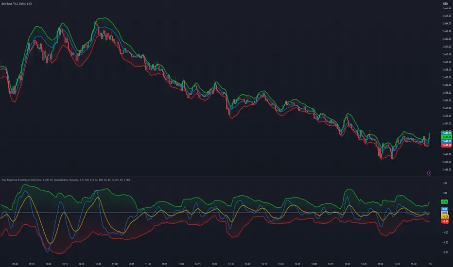
Hybrid Adaptive Double Exponential Smoothing🙏🏻 This is HADES (Hybrid Adaptive Double Exponential Smoothing) : fully data-driven & adaptive exponential smoothing method, that gains all the necessary info directly from data in the most natural way and needs no subjective parameters & no optimizations. It gets applied to data itself -> to fit residuals & one-point forecast errors, all at O(1) algo complexity. I designed it for streaming high-frequency univariate time series data, such as medical sensor readings, orderbook data, tick charts, requests generated by a backend, etc.
The HADES method is:
fit & forecast = a + b * (1 / alpha + T - 1)
T = 0 provides in-sample fit for the current datum, and T + n provides forecast for n datapoints.
y = input time series
a = y, if no previous data exists
b = 0, if no previous data exists
otherwise:
a = alpha * y + (1 - alpha) * a
b = alpha * (a - a ) + (1 - alpha) * b
alpha = 1 / sqrt(len * 4)
len = min(ceil(exp(1 / sig)), available data)
sig = sqrt(Absolute net change in y / Sum of absolute changes in y)
For the start datapoint when both numerator and denominator are zeros, we define 0 / 0 = 1
...
The same set of operations gets applied to the data first, then to resulting fit absolute residuals to build prediction interval, and finally to absolute forecasting errors (from one-point ahead forecast) to build forecasting interval:
prediction interval = data fit +- resoduals fit * k
forecasting interval = data opf +- errors fit * k
where k = multiplier regulating intervals width, and opf = one-point forecasts calculated at each time t
...
How-to:
0) Apply to your data where it makes sense, eg. tick data;
1) Use power transform to compensate for multiplicative behavior in case it's there;
2) If you have complete data or only the data you need, like the full history of adjusted close prices: go to the next step; otherwise, guided by your goal & analysis, adjust the 'start index' setting so the calculations will start from this point;
3) Use prediction interval to detect significant deviations from the process core & make decisions according to your strategy;
4) Use one-point forecast for nowcasting;
5) Use forecasting intervals to ~ understand where the next datapoints will emerge, given the data-generating process will stay the same & lack structural breaks.
I advise k = 1 or 1.5 or 4 depending on your goal, but 1 is the most natural one.
...
Why exponential smoothing at all? Why the double one? Why adaptive? Why not Holt's method?
1) It's O(1) algo complexity & recursive nature allows it to be applied in an online fashion to high-frequency streaming data; otherwise, it makes more sense to use other methods;
2) Double exponential smoothing ensures we are taking trends into account; also, in order to model more complex time series patterns such as seasonality, we need detrended data, and this method can be used to do it;
3) The goal of adaptivity is to eliminate the window size question, in cases where it doesn't make sense to use cumulative moving typical value;
4) Holt's method creates a certain interaction between level and trend components, so its results lack symmetry and similarity with other non-recursive methods such as quantile regression or linear regression. Instead, I decided to base my work on the original double exponential smoothing method published by Rob Brown in 1956, here's the original source , it's really hard to find it online. This cool dude is considered the one who've dropped exponential smoothing to open access for the first time🤘🏻
R&D; log & explanations
If you wanna read this, you gotta know, you're taking a great responsability for this long journey, and it gonna be one hell of a trip hehe
Machine learning, apprentissage automatique, машинное обучение, digital signal processing, statistical learning, data mining, deep learning, etc., etc., etc.: all these are just artificial categories created by the local population of this wonderful world, but what really separates entities globally in the Universe is solution complexity / algorithmic complexity.
In order to get the game a lil better, it's gonna be useful to read the HTES script description first. Secondly, let me guide you through the whole R&D; process.
To discover (not to invent) the fundamental universal principle of what exponential smoothing really IS, it required the review of the whole concept, understanding that many things don't add up and don't make much sense in currently available mainstream info, and building it all from the beginning while avoiding these very basic logical & implementation flaws.
Given a complete time t, and yet, always growing time series population that can't be logically separated into subpopulations, the very first question is, 'What amount of data do we need to utilize at time t?'. Two answers: 1 and all. You can't really gain much info from 1 datum, so go for the second answer: we need the whole dataset.
So, given the sequential & incremental nature of time series, the very first and basic thing we can do on the whole dataset is to calculate a cumulative , such as cumulative moving mean or cumulative moving median.
Now we need to extend this logic to exponential smoothing, which doesn't use dataset length info directly, but all cool it can be done via a formula that quantifies the relationship between alpha (smoothing parameter) and length. The popular formulas used in mainstream are:
alpha = 1 / length
alpha = 2 / (length + 1)
The funny part starts when you realize that Cumulative Exponential Moving Averages with these 2 alpha formulas Exactly match Cumulative Moving Average and Cumulative (Linearly) Weighted Moving Average, and the same logic goes on:
alpha = 3 / (length + 1.5) , matches Cumulative Weighted Moving Average with quadratic weights, and
alpha = 4 / (length + 2) , matches Cumulative Weighted Moving Average with cubic weghts, and so on...
It all just cries in your shoulder that we need to discover another, native length->alpha formula that leverages the recursive nature of exponential smoothing, because otherwise, it doesn't make sense to use it at all, since the usual CMA and CMWA can be computed incrementally at O(1) algo complexity just as exponential smoothing.
From now on I will not mention 'cumulative' or 'linearly weighted / weighted' anymore, it's gonna be implied all the time unless stated otherwise.
What we can do is to approach the thing logically and model the response with a little help from synthetic data, a sine wave would suffice. Then we can think of relationships: Based on algo complexity from lower to higher, we have this sequence: exponential smoothing @ O(1) -> parametric statistics (mean) @ O(n) -> non-parametric statistics (50th percentile / median) @ O(n log n). Based on Initial response from slow to fast: mean -> median Based on convergence with the real expected value from slow to fast: mean (infinitely approaches it) -> median (gets it quite fast).
Based on these inputs, we need to discover such a length->alpha formula so the resulting fit will have the slowest initial response out of all 3, and have the slowest convergence with expected value out of all 3. In order to do it, we need to have some non-linear transformer in our formula (like a square root) and a couple of factors to modify the response the way we need. I ended up with this formula to meet all our requirements:
alpha = sqrt(1 / length * 2) / 2
which simplifies to:
alpha = 1 / sqrt(len * 8)
^^ as you can see on the screenshot; where the red line is median, the blue line is the mean, and the purple line is exponential smoothing with the formulas you've just seen, we've met all the requirements.
Now we just have to do the same procedure to discover the length->alpha formula but for double exponential smoothing, which models trends as well, not just level as in single exponential smoothing. For this comparison, we need to use linear regression and quantile regression instead of the mean and median.
Quantile regression requires a non-closed form solution to be solved that you can't really implement in Pine Script, but that's ok, so I made the tests using Python & sklearn:
paste.pics
^^ on this screenshot, you can see the same relationship as on the previous screenshot, but now between the responses of quantile regression & linear regression.
I followed the same logic as before for designing alpha for double exponential smoothing (also considered the initial overshoots, but that's a little detail), and ended up with this formula:
alpha = sqrt(1 / length) / 2
which simplifies to:
alpha = 1 / sqrt(len * 4)
Btw, given the pattern you see in the resulting formulas for single and double exponential smoothing, if you ever want to do triple (not Holt & Winters) exponential smoothing, you'll need len * 2 , and just len * 1 for quadruple exponential smoothing. I hope that based on this sequence, you see the hint that Maybe 4 rounds is enough.
Now since we've dealt with the length->alpha formula, we can deal with the adaptivity part.
Logically, it doesn't make sense to use a slower-than-O(1) method to generate input for an O(1) method, so it must be something universal and minimalistic: something that will help us measure consistency in our data, yet something far away from statistics and close enough to topology.
There's one perfect entity that can help us, this is fractal efficiency. The way I define fractal efficiency can be checked at the very beginning of the post, what matters is that I add a square root to the formula that is not typically added.
As explained in the description of my metric QSFS , one of the reasons for SQRT-transformed values of fractal efficiency applied in moving window mode is because they start to closely resemble normal distribution, yet with support of (0, 1). Data with this interesting property (normally distributed yet with finite support) can be modeled with the beta distribution.
Another reason is, in infinitely expanding window mode, fractal efficiency of every time series that exhibits randomness tends to infinitely approach zero, sqrt-transform kind of partially neutralizes this effect.
Yet another reason is, the square root might better reflect the dimensional inefficiency or degree of fractal complexity, since it could balance the influence of extreme deviations from the net paths.
And finally, fractals exhibit power-law scaling -> measures like length, area, or volume scale in a non-linear way. Adding a square root acknowledges this intrinsic property, while connecting our metric with the nature of fractals.
---
I suspect that, given analogies and connections with other topics in geometry, topology, fractals and most importantly positive test results of the metric, it might be that the sqrt transform is the fundamental part of fractal efficiency that should be applied by default.
Now the last part of the ballet is to convert our fractal efficiency to length value. The part about inverse proportionality is obvious: high fractal efficiency aka high consistency -> lower window size, to utilize only the last data that contain brand new information that seems to be highly reliable since we have consistency in the first place.
The non-obvious part is now we need to neutralize the side effect created by previous sqrt transform: our length values are too low, and exponentiation is the perfect candidate to fix it since translating fractal efficiency into window sizes requires something non-linear to reflect the fractal dynamics. More importantly, using exp() was the last piece that let the metric shine, any other transformations & formulas alike I've tried always had some weird results on certain data.
That exp() in the len formula was the last piece that made it all work both on synthetic and on real data.
^^ a standalone script calculating optimal dynamic window size
Omg, THAT took time to write. Comment and/or text me if you need
...
"Versace Pip-Boy, I'm a young gun coming up with no bankroll" 👻
∞
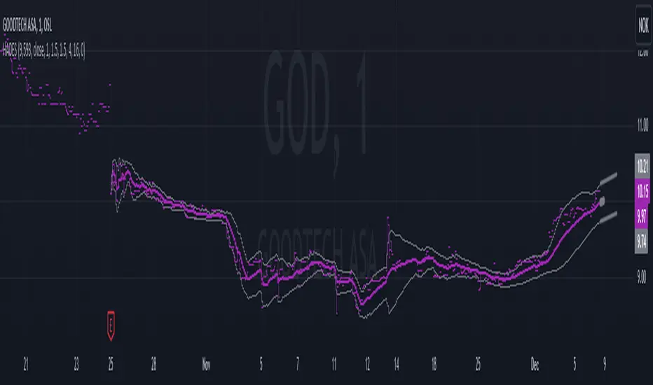
Fourier Extrapolation of PriceThis advanced algorithm leverages Fourier analysis to predict price trends by decomposing historical price data into its frequency components. Unlike traditional algorithms that often operate in lower-dimensional spaces, this method harnesses a multidimensional approach to capture intricate market behaviors. By utilizing additional dimensions, the algorithm identifies and extrapolates subtle patterns and oscillations that are typically overlooked, providing a more robust and nuanced forecast.
Ideal for traders seeking a deeper understanding of market dynamics, this tool offers an enhanced predictive capability by aligning its calculations with the complexity of real-world financial systems.

Volume Based Price Prediction [EdgeTerminal]This indicator combines price action, volume analysis, and trend prediction to forecast potential future price movements. The indicator creates a dynamic prediction zone with confidence bands, helping you visualize possible price trajectories based on current market conditions.
Key Features
Dynamic price prediction based on volume-weighted trend analysis
Confidence bands showing potential price ranges
Volume-based candle coloring for enhanced market insight
VWAP and Moving Average overlay
Customizable prediction parameters
Real-time updates with each new bar
Technical Components:
Volume-Price Correlation: The indicator analyzes the relationship between price movements and volume, Identifies stronger trends through volume confirmation and uses Volume-Weighted Average Price (VWAP) for price equilibrium
Trend Strength Analysis: Calculates trend direction using exponential moving averages, weights trend strength by relative volume and incorporates momentum for improved accuracy
Prediction Algorithm: combines current price, trend, and volume metrics, projects future price levels using weighted factors and generates confidence bands based on price volatility
Customizable Parameters:
Moving Average Length: Controls the smoothing period for calculations
Volume Weight Factor: Adjusts how much volume influences predictions
Prediction Periods: Number of bars to project into the future
Confidence Band Width: Controls the width of prediction bands
How to use it:
Look for strong volume confirmation with green candles, watch for prediction line slope changes, use confidence bands to gauge potential volatility and compare predictions with key support/resistance levels
Some useful tips:
Start with default settings and adjust gradually
Use wider confidence bands in volatile markets
Consider prediction lines as zones rather than exact levels
Best applications of this indicator:
Trend continuation probability assessment
Potential reversal point identification
Risk management through confidence bands
Volume-based trend confirmation
MACD Cloud with Moving Average and ATR BandsThe algorithm implements a technical analysis indicator that combines the MACD Cloud, Moving Averages (MA), and volatility bands (ATR) to provide signals on market trends and potential reversal points. It is divided into several sections:
🎨 Color Bars:
Activated based on user input.
Controls bar color display according to price relative to ATR levels and moving average (MA).
Logic:
⚫ Black: Potential bearish reversal (price above the upper ATR band).
🔵 Blue: Potential bullish reversal (price below the lower ATR band).
o
🟢 Green: Bullish trend (price between the MA and upper ATR band).
o
🔴 Red: Bearish trend (price between the lower ATR band and MA).
o
📊 MACD Bars:
Description:
The MACD Bars section is activated by default and can be modified based on user input.
🔴 Red: Indicates a bearish trend, shown when the MACD line is below the Signal line (Signal line is a moving average of MACD).
🔵 Blue: Indicates a bullish trend, shown when the MACD line is above the Signal line.
Matching colors between MACD Bars and MACD Cloud visually confirms trend direction.
MACD Cloud Logic: The MACD Cloud is based on Moving Average Convergence Divergence (MACD), a momentum indicator showing the relationship between two moving averages of price.
MACD and Signal Lines: The cloud visualizes the MACD line relative to the Signal line. If the MACD line is above the Signal line, it indicates a potential bullish trend, while below it suggests a potential bearish trend.
☁️ MA Cloud:
The MA Cloud uses three moving averages to analyze price direction:
Moving Average Relationship: Three MAs of different periods are plotted. The cloud turns green when the shorter MA is above the longer MA, indicating an uptrend, and red when below, suggesting a downtrend.
Trend Visualization: This graphical representation shows the trend direction.
📉 ATR Bands:
The ATR bands calculate overbought and oversold limits using a weighted moving average (WMA) and ATR.
Center (matr): Shows general trend; prices above suggest an uptrend, while below indicate a downtrend.
Up ATR 1: Marks the first overbought level, suggesting a potential bearish reversal if the price moves above this band.
Down ATR 1: Marks the first oversold level, suggesting a possible bullish reversal if the price moves below this band.
Up ATR 2: Extends the overbought range to an extreme, reinforcing the possibility of a bearish reversal at this level.
Down ATR 2: Extends the oversold range to an extreme, indicating a stronger bullish reversal possibility if price reaches here.
Español:
El algoritmo implementa un indicador de análisis técnico que combina la nube MACD, promedios móviles (MA) y bandas de volatilidad (ATR) para proporcionar señales sobre tendencias del mercado y posibles puntos de reversión. Se divide en varias secciones:
🎨 Barras de Color:
- Activado según la entrada del usuario.
- Controla la visualización del color de las barras según el precio en relación con los niveles de ATR y el promedio móvil (MA).
- **Lógica:**
- ⚫ **Negro**: Reversión bajista potencial (precio por encima de la banda superior ATR).
- 🔵 **Azul**: Reversión alcista potencial (precio por debajo de la banda inferior ATR).
- 🟢 **Verde**: Tendencia alcista (precio entre el MA y la banda superior ATR).
- 🔴 **Rojo**: Tendencia bajista (precio entre la banda inferior ATR y el MA).
### 📊 Barras MACD:
- **Descripción**:
- La sección de barras MACD se activa por defecto y puede modificarse según la entrada del usuario.
- 🔴 **Rojo**: Indica una tendencia bajista, cuando la línea MACD está por debajo de la línea de señal (la línea de señal es una media móvil de la MACD).
- 🔵 **Azul**: Indica una tendencia alcista, cuando la línea MACD está por encima de la línea de señal.
- La coincidencia de colores entre las barras MACD y la nube MACD confirma visualmente la dirección de la tendencia.
### 🌥️ Nube MACD:
- **Lógica de la Nube MACD**: Basada en el indicador de convergencia-divergencia de medias móviles (MACD), que muestra la relación entre dos medias móviles del precio.
- **Líneas MACD y de Señal**: La nube visualiza la relación entre la línea MACD y la línea de señal. Si la línea MACD está por encima de la de señal, indica una tendencia alcista potencial; si está por debajo, sugiere una tendencia bajista.
### ☁️ Nube MA:
- **Relación entre Medias Móviles**: Se trazan tres medias móviles de diferentes períodos. La nube se vuelve verde cuando la media más corta está por encima de la más larga, indicando una tendencia alcista, y roja cuando está por debajo, sugiriendo una tendencia bajista.
- **Visualización de Tendencias**: Proporciona una representación gráfica de la dirección de la tendencia.
### 📉 Bandas ATR:
- Las bandas ATR calculan límites de sobrecompra y sobreventa usando una media ponderada y el ATR.
- **Centro (matr)**: Muestra la tendencia general; precios por encima indican tendencia alcista y debajo, bajista.
- **Up ATR 1**: Marca el primer nivel de sobrecompra, sugiriendo una reversión bajista potencial si el precio sube por encima de esta banda.
- **Down ATR 1**: Marca el primer nivel de sobreventa, sugiriendo una reversión alcista potencial si el precio baja por debajo de esta banda.
- **Up ATR 2**: Amplía el rango de sobrecompra a un nivel extremo, reforzando la posibilidad de reversión bajista.
- **Down ATR 2**: Extiende el rango de sobreventa a un nivel extremo, sugiriendo una reversión alcista más fuerte si el precio alcanza esta banda.
Third-order moment by TonymontanovThe "Third-order moment" indicator is designed to help traders identify asymmetries and potential turning points in a financial instrument's price distribution over a specified period. By calculating the skewness of the price distribution, this indicator provides insights into the potential future movement direction of the market.
User Parameters:
- Length: This parameter defines the number of bars (or periods) used to compute the mean and third-order moment. A longer length provides a broader historical context, which may smooth out short-term volatility.
- Source: The data input for calculations, defaulting to the closing price of each bar, although users can select alternatives like open, high, low, or any custom value to suit their analysis preferences.
Operational Algorithm:
1. Mean Calculation:
- The indicator begins by calculating the arithmetic mean of the selected data source over the specified period.
2. Third-order Moment Calculation:
- A deviation from the mean is calculated for each data point. These deviations are then cubed to capture any asymmetry in the price distribution.
- The third-order moment is determined by summing these cubed deviations over the specified length and dividing by the number of periods, providing a measure of skewness.
3. Graphical Representation:
- The indicator plots the third-order moment as a column plot. The color of the columns changes based on the sign of the moment: green for positive and red for negative, suggesting bullish and bearish skewness, respectively.
- A zero line is included to help visualize transitions between positive and negative skewness clearly.
- Additionally, the background color shifts depending on whether the third-order moment is above or below zero, further highlighting the prevailing market sentiment.
The "Third-order moment" indicator is a valuable tool for traders looking to gauge the market's skewness, helping identify potential trend continuations or reversals. By understanding the dominance of positive or negative skewness, traders can make more informed decisions.
Asymmetric volatilityThe "Asymmetric Volatility" indicator is designed to visualize the differences in volatility between upward and downward price movements of a selected instrument. It operates on the principle of analyzing price movements over a specified time period, with particular focus on the symmetrical evaluation of both price rises and falls.
User Parameters:
- Length: This parameter specifies the number of bars (candles) used to calculate the average volatility. The larger the value, the longer the time period, and the smoother the volatility data will be.
- Source: This represents the input data for the indicator calculations. By default, the close value of each bar is used, but the user can choose another data source (such as open, high, low, or any custom value).
Operational Algorithm:
1. Movement Calculation:
- UpMoves: Computed as the positive difference between the current bar value and the previous bar value, if it is greater than zero.
- DownMoves: Computed as the positive difference between the previous bar value and the current bar value, if it is greater than zero.
2. Volatility Calculation:
- UpVolatility: This is the arithmetic mean of the UpMoves values over the specified period.
- DownVolatility: This is the arithmetic mean of the DownMoves values over the specified period.
3. Graphical Representation:
- The indicator displays two plots: upward and downward volatility, represented by green and red lines, respectively.
- The background color changes based on which volatility is dominant: a green background indicates that upward volatility prevails, while a red background indicates downward volatility.
The indicator allows traders to quickly assess in which direction the market is more volatile at the moment, which can be useful for making trading decisions and evaluating the current market situation.
Stationarity Test: Dickey-Fuller & KPSS [Pinescriptlabs]
📊 Kwiatkowski-Phillips-Schmidt-Shin Model Indicator & Dickey-Fuller Test 📈
This algorithm performs two statistical tests on the price spread between two selected instruments: the first from the current chart and the second determined in the settings. The purpose is to determine if their relationship is stationary. It then uses this information to generate **visual signals** based on how far the current relationship deviates from its historical average.
⚙️ Key Components:
• 🧪 ADF Test (Augmented Dickey-Fuller):** Checks if the spread between the two instruments is stationary.
• 🔬 KPSS Test (Kwiatkowski-Phillips-Schmidt-Shin):** Another test for stationarity, complementing the ADF test.
• 📏 Z-Score Calculation:** Measures how many standard deviations the current spread is from its historical mean.
• 📊 Dynamic Threshold:** Adjusts the trading signal threshold based on recent market volatility.
🔍 What the Values Mean:
The indicator displays several key values in a table:
• 📈 ADF Stationarity:** Shows "Stationary" or "Non-Stationary" based on the ADF test result.
• 📉 KPSS Stationarity:** Shows "Stationary" or "Non-Stationary" based on the KPSS test result.
• 📏 Current Z-Score:** The current Z-score of the spread.
• 🔗 Hedge Ratio:** The relationship coefficient between the two instruments.
• 🌐 Market State:** Describes the current market condition based on the Z-score.
📊 How to Interpret the Chart:
• The main chart displays the Z-score of the spread over time.
• The green and red lines represent the upper and lower thresholds for trading signals.
• The area between the **Z-score** and the thresholds is filled when a trading signal is active.
• Additional charts show the **statistics of the ADF and KPSS tests** and their critical values.
**📉 Practical Example: NVIDIA Corporation (NVDA)**
Looking at the chart for **NVIDIA Corporation (NVDA)**, we can see how the indicator applies in a real case:
1. **Main Chart (Top):**
• Shows the **historical price** of NVIDIA on a weekly scale.
• A general **uptrend** is observed with periods of consolidation.
2. **KPSS & ADF Indicator (Bottom):**
• The lower chart shows the KPSS & ADF Model indicator applied to NVIDIA.
• The **green line** represents the Z-score of the spread.
• The **green shaded areas** indicate periods where the Z-score exceeded the thresholds, generating trading signals.
3. **📋 Current Values in the Table:**
• **ADF Stationarity:** Non-Stationary
• **KPSS Stationarity:** Non-Stationary
• **Current Z-Score:** 3.45
• **Hedge Ratio:** -164.8557
• **Market State:** Moderate Volatility
4. **🔍 Interpretation:**
• A Z-score of **3.45** suggests that NVIDIA’s price is significantly above its historical average relative to **EURUSD**.
• Both the **ADF** and **KPSS** tests indicate **non-stationarity**, suggesting **caution** when using mean reversion signals at this moment.
• The market state "Moderate Volatility" indicates noticeable deviation, but not extreme.
---
**💡 Usage:**
• **When Both Tests Show Stationarity:**
• **🔼 If Z-score > Upper Threshold:** Consider **buying the first instrument** and **selling the second**.
• **🔽 If Z-score < Lower Threshold:** Consider **selling the first instrument** and **buying the second**.
• **When Either Test Shows Non-Stationarity:**
• Wait for the relationship to become **stationary** before trading.
• **Market State:**
• Use this information to evaluate **general market conditions** and adjust your trading strategy accordingly.
**Mirror Comparison of the Same as Symbol 2 🔄📊**
**📊 Table Values:**
• **Extreme Volatility Threshold:** This value is displayed when the **Z-score** exceeds **100%**, indicating **extreme deviation**. It signals a potential **trading opportunity**, as the spread has reached unusually high or low levels, suggesting a **reversion or correction** in the market.
• **Mean Reversion Threshold:** Appears when the **Z-score** begins returning towards the mean after a period of **high or extreme volatility**. It indicates that the spread between the assets is returning to normal levels, suggesting a phase of **stabilization**.
• **Neutral Zone:** Displayed when the **Z-score** is near **zero**, signaling that the spread between assets is within expected limits. This indicates a **balanced market** with no significant volatility or clear trading opportunities.
• **Low Volatility Threshold:** Appears when the **Z-score** is below **70%** of the dynamic threshold, reflecting a period of **low volatility** and market stability, indicating fewer trading opportunities.
Español:
📊 Indicador del Modelo Kwiatkowski-Phillips-Schmidt-Shin & Prueba de Dickey-Fuller 📈
Este algoritmo realiza dos pruebas estadísticas sobre la diferencia de precios (spread) entre dos instrumentos seleccionados: el primero en el gráfico actual y el segundo determinado en la configuración. El objetivo es determinar si su relación es estacionaria. Luego utiliza esta información para generar señales visuales basadas en cuánto se desvía la relación actual de su promedio histórico.
⚙️ Componentes Clave:
• 🧪 Prueba ADF (Dickey-Fuller Aumentada): Verifica si el spread entre los dos instrumentos es estacionario.
• 🔬 Prueba KPSS (Kwiatkowski-Phillips-Schmidt-Shin): Otra prueba para la estacionariedad, complementando la prueba ADF.
• 📏 Cálculo del Z-Score: Mide cuántas desviaciones estándar se encuentra el spread actual de su media histórica.
• 📊 Umbral Dinámico: Ajusta el umbral de la señal de trading en función de la volatilidad reciente del mercado.
🔍 Qué Significan los Valores:
El indicador muestra varios valores clave en una tabla:
• 📈 Estacionariedad ADF: Muestra "Estacionario" o "No Estacionario" basado en el resultado de la prueba ADF.
• 📉 Estacionariedad KPSS: Muestra "Estacionario" o "No Estacionario" basado en el resultado de la prueba KPSS.
• 📏 Z-Score Actual: El Z-score actual del spread.
• 🔗 Ratio de Cobertura: El coeficiente de relación entre los dos instrumentos.
• 🌐 Estado del Mercado: Describe la condición actual del mercado basado en el Z-score.
📊 Cómo Interpretar el Gráfico:
• El gráfico principal muestra el Z-score del spread a lo largo del tiempo.
• Las líneas verdes y rojas representan los umbrales superior e inferior para las señales de trading.
• El área entre el Z-score y los umbrales se llena cuando una señal de trading está activa.
• Los gráficos adicionales muestran las estadísticas de las pruebas ADF y KPSS y sus valores críticos.
📉 Ejemplo Práctico: NVIDIA Corporation (NVDA)
Observando el gráfico para NVIDIA Corporation (NVDA), podemos ver cómo se aplica el indicador en un caso real:
Gráfico Principal (Superior): • Muestra el precio histórico de NVIDIA en escala semanal. • Se observa una tendencia alcista general con períodos de consolidación.
Indicador KPSS & ADF (Inferior): • El gráfico inferior muestra el indicador Modelo KPSS & ADF aplicado a NVIDIA. • La línea verde representa el Z-score del spread. • Las áreas sombreadas en verde indican períodos donde el Z-score superó los umbrales, generando señales de trading.
📋 Valores Actuales en la Tabla: • Estacionariedad ADF: No Estacionario • Estacionariedad KPSS: No Estacionario • Z-Score Actual: 3.45 • Ratio de Cobertura: -164.8557 • Estado del Mercado: Volatilidad Moderada
🔍 Interpretación: • Un Z-score de 3.45 sugiere que el precio de NVIDIA está significativamente por encima de su promedio histórico en relación con EURUSD. • Tanto la prueba ADF como la KPSS indican no estacionariedad, lo que sugiere precaución al usar señales de reversión a la media en este momento. • El estado del mercado "Volatilidad Moderada" indica una desviación notable, pero no extrema.
💡 Uso:
• Cuando Ambas Pruebas Muestran Estacionariedad:
• 🔼 Si Z-score > Umbral Superior: Considera comprar el primer instrumento y vender el segundo.
• 🔽 Si Z-score < Umbral Inferior: Considera vender el primer instrumento y comprar el segundo.
• Cuando Alguna Prueba Muestra No Estacionariedad:
• Espera a que la relación se vuelva estacionaria antes de operar.
• Estado del Mercado:
• Usa esta información para evaluar las condiciones generales del mercado y ajustar tu estrategia de trading en consecuencia.
Comparativo en Espejo del Mismo Como Símbolo 2 🔄📊
📊 Valores de la Tabla:
• Umbral de Volatilidad Extrema: Este valor se muestra cuando el Z-score supera el 100%, indicando desviación extrema. Señala una posible oportunidad de trading, ya que el spread entre los activos ha alcanzado niveles inusualmente altos o bajos, lo que podría indicar una reversión o corrección en el mercado.
• Umbral de Reversión a la Media: Aparece cuando el Z-score comienza a volver hacia la media tras un período de alta o extrema volatilidad. Indica que el spread entre los activos está regresando a niveles normales, sugiriendo una fase de estabilización.
• Zona Neutral: Se muestra cuando el Z-score está cerca de cero, señalando que el spread entre activos está dentro de lo esperado. Esto indica un mercado equilibrado con ninguna volatilidad significativa ni oportunidades claras de trading.
• Umbral de Baja Volatilidad: Aparece cuando el Z-score está por debajo del 70% del umbral dinámico, reflejando un período de baja volatilidad y estabilidad del mercado, indicando menos oportunidades de trading.

Smoothed SuperTrend with VWAP Confirmation [CHE] Smoothed SuperTrend with Automated Optimization and VWAP Confirmation
Overview
The "Smoothed SuperTrend with VWAP Confirmation" is an advanced technical analysis indicator designed for precise trend identification and trading signal generation. This script integrates a smoothed version of the popular SuperTrend indicator with an additional layer of confirmation using the Volume-Weighted Average Price (VWAP). The combination of these two elements offers traders a powerful tool for identifying optimal entry and exit points in the market.
Key Features
1. Smoothed SuperTrend
- Super Smoother Algorithm: The SuperTrend in this script is not just a regular one; it is enhanced by the Super Smoother filter, which reduces market noise and provides more reliable trend signals.
- Customizable Parameters: Traders can adjust three different sets of SuperTrend parameters (factor and ATR length), allowing them to tailor the indicator to their specific trading strategies.
- Automatic Optimization: The script automatically evaluates the performance of each SuperTrend parameter set and selects the one with the best cumulative performance. This selection process can be set to pick either the best or the worst performing parameter set, depending on the trader's preference.
2. VWAP Confirmation
- Precise Trend Confirmation: Once the best-performing SuperTrend is identified, the script further refines the signals by using VWAP as a confirmation tool. VWAP is a highly respected indicator in the trading community, often used to assess the true average price of an asset.
- Long and Short Signal Generation: The script generates Long and Short signals only when the price action is confirmed by both the SuperTrend and VWAP. For a Long signal, the price must be above the VWAP, and for a Short signal, it must be below the VWAP. This dual confirmation ensures higher accuracy and reduces the likelihood of false signals.
3. Visual and Informative Labels
- Signal Labels: Upon confirmation of a trend reversal by both the SuperTrend and VWAP, the script plots clear labels on the chart, indicating confirmed Long or Short signals. These labels are customizable in terms of color, text, and size, ensuring they fit seamlessly into any chart setup.
- Best Parameters Display: At the close of the most recent bar, the script displays a label that provides detailed information about the best-performing SuperTrend parameters and their cumulative performance. This feature keeps traders informed about which settings are currently most effective.
Input Customization Options
1. Super Smoother Length
- Traders can define the length of the Super Smoother filter, which is used to smooth both price data and ATR (Average True Range) values. This input allows traders to control the sensitivity of the indicator, with shorter lengths providing faster responses and longer lengths offering smoother trends.
2. SuperTrend Parameters
- Factor: For each of the three SuperTrends, traders can set a unique factor that determines the distance of the SuperTrend bands from the average price. A higher factor results in wider bands and fewer signals, while a lower factor results in narrower bands and more signals.
- ATR Length: Traders can also specify the length of the ATR used in each SuperTrend calculation. A longer ATR period captures broader market volatility, while a shorter period focuses on more immediate price movements.
3. Label Settings
- Label Colors: The script allows full customization of label colors for Long and Short signals, ensuring that they match the trader’s chart aesthetics.
- Label Text Colors and Sizes: Traders can adjust the text color and size of the labels for Long, Short, and information labels, allowing them to prioritize visibility and readability on their charts.
4. Performance Selection Mode
- Best or Worst Performer: This input allows traders to select whether the script should optimize for the best or worst performing SuperTrend parameter set. This flexibility is useful in different market conditions, where a trader might want to analyze either the strongest trend or focus on a contrarian strategy.
5. VWAP Calculation
- The script automatically recalculates the VWAP based on trend changes, ensuring that the confirmation signals are as accurate and relevant as possible to the current market context.
Important Note
This script is designed to provide more accurate trend signals and confirmations, but like all technical indicators, it should not be used in isolation. It is recommended to use this tool as part of a broader trading strategy, including proper risk management and consideration of fundamental market conditions.
Conclusion
The "Smoothed SuperTrend with VWAP Confirmation" script is an innovative trading tool that combines the strengths of the SuperTrend and VWAP indicators. By integrating smoothing techniques and automatic parameter optimization, this indicator provides traders with more accurate and reliable trend signals. The added confirmation by VWAP further enhances the precision of the entry and exit points, making it an excellent choice for traders looking to improve their technical analysis and trading outcomes. This tool is especially valuable for those who prefer customizable inputs and a systematic approach to trading, ensuring that the indicator adapts to various market conditions and individual trading styles.
Best regards
Chervolino
