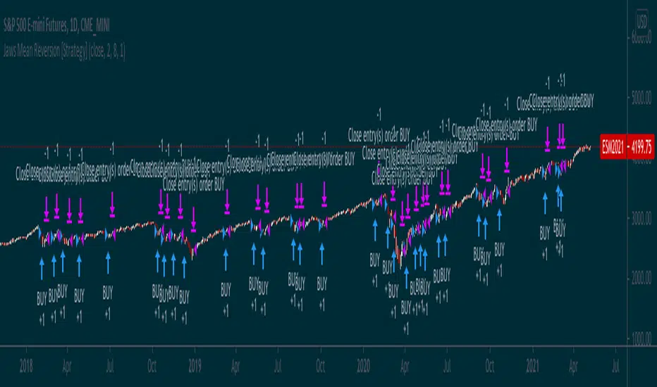
Jaws Mean Reversion [Strategy]This very simple strategy is an implementation of PJ Sutherlands' Jaws Mean reversion algorithm. It simply buys when a small moving average period (e.g. 2) is below
a longer moving average period (e.g. 5) by a certain percentage and closes when the small period average crosses over the longer moving average.
If you are going to use this, you may wish to apply this to a range of investment assets using a screener for setups, as the amount signals are low. Alternatively, you may wish to tweak the settings to provide more signals.
Context can be found here:
LINK
ابحث في النصوص البرمجية عن "algo"
(JS) Multi-Time Frame Pivot Point Detector 2.0So here's an updated version of my automatic Pivot Point detector.
If you don't like having a bunch of Pivots on your chart at once, or having to cycle through various resolutions to see different ones, this is for you!
What does this indicator do? It automatically detects the nearest daily, weekly, and monthly pivot points both above and below the current price and automatically plots them for you. It's really just as simple as that.
You select how far back you want it to plot with the "Pivot Point Look Back Period" option.
I also have transparency options for each type of pivot so its easy to find the opacity you prefer and save it as a default setting.
With "Turn Off Each Pivot Point On All Time Frames" turned on, as an example, if you were to uncheck "S1/R1" then it turns S1/R1 plots off across all 3 pivot resolutions. By default however, I have it set where you can pick and choose each one individually.
I also added the default "VWAP Periodic" script from TradingView in there with it (not in prior version). This works identical to the built in indicator (because it is identical).
Trading algorithms like to target pivot points and liquidity, so I figured they would pair together nicely for active trading.
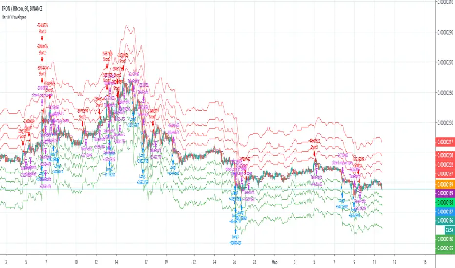
HatiKO EnvelopesPublished source code is subject to the terms of the GNU Affero General Public License v3.0
This script describes and provides backtesting functionality to internal strategy of algorithmic crypto trading software "HatiKO bot".
Suitable for backtesting any Cryptocurrency Pair on any Exchange/Platform, any Timeframe.
Core Mechanics of this strategy are based on theory of price always returning to Moving Average + Envelopes indicator (Moving_average_envelope from Wiki)
Developement of this script and trading software is inspired by:
"Essential Technical Analysis: Tools and Techniques to Spot Market Trends" by Leigh Stevens (published on 12th of April 2002)
"Moving Average Envelopes" by ChartSchool, StockCharts platform (published on 13th of April 2015 or earlier)
"Коля Колеснік" from Crypto Times channel ("Метод сетка", published on 19th of August 2018)
"3 ways to use Moving Average Envelopes" by Rich Fitton, published on Trader's Nest (published on 28st of November 2018 or earlier)
noro's "Robot WhiteBox ShiftMA" strategy v1 script, published on TradingView platform (published on 29th of August 2018)
"Moving Average Envelopes: A Popular Trading Tool" Investopedia article (published 25th of June 2019)
and KROOL1980's blogpost on Argolabs ("Гридерство или Сетка как источник прибыли на форекс", published on 27th of February 2015)
Core Features:
1) Up to 4 Envelopes in each direction (Long/Short)
2) Use any of 6 different basis MAs, optionally use different MAs for Opening and Closure
3) Use different Timeframes for MA calculation, without any repainting and lookahead bias.
4) Fixed order size, not Martingale strategy
5) Close open position earlier by using Deviation parameter
6) PineScript v4 code
Options description:
Lot - % from your initial balance to use for order size calculation
Timeframe Short - Timeframe to use for Short Opening MA calculation, can be chosen from dropdown list, default is Current Graph Timeframe
MA Type Short - Type of MA to use for Short Opening MA calculation, can be chosen from dropdown list, default is SMA
Data Short - Source of Price for Short Opening MA calculation, can be chosen from dropdown list, default is OHLC4
MA Length Short - Period used for Short Opening MA calculation, should be >=1, default is 3
MA offset Short - Offset for MA value used for Short Envelopes calculation, should be >= 0, default is 0
Timeframe Long - Timeframe to use for Long Opening MA calculation, can be chosen from dropdown list, default is Current Graph Timeframe
MA Type Long - Type of MA to use for Long Opening MA calculation, can be chosen from dropdown list, default is SMA
Data Long - Source of Price for Long Opening MA calculation, can be chosen from dropdown list, default is OHLC4
MA Length Long - Period used for Long Opening MA calculation, should be >=1, default is 3
MA offset Long - Offset for MA value used for Long Envelopes calculation, should be >= 0, default is 0
Mode close MA Short - Enable different MA for Short position Closure, default is "false". If false, Closure MA = Opening MA
Timeframe Short Close - Timeframe to use for Short Position Closure MA calculation, can be chosen from dropdown list, default is Current Graph Timeframe
MA Type Close Short - Type of MA to use for Short Position Closure MA calculation, can be chosen from dropdown list, default is SMA
Data Short Close - Source of Price for Short Closure MA calculation, can be chosen from dropdown list, default is OHLC4
MA Length Short Close - Period used for Short Opening MA calculation, should be >=1, default is 3
Short Deviation - % to move from MA value, used to close position above or beyond MA, can be negative, default is 0
MA offset Short Close - Offset for MA value used for Short Position Closure calculation, should be >= 0, default is 0
Mode close MA Long - Enable different MA for Long position Closure, default is "false". If false, Closure MA = Opening MA
Timeframe Long Close - Timeframe to use for Long Position Closure MA calculation, can be chosen from dropdown list, default is Current Graph Timeframe
MA Type Close Long - Type of MA to use for Long Position Closure MA calculation, can be chosen from dropdown list, default is SMA
Data Long Close - Source of Price for Long Closure MA calculation, can be chosen from dropdown list, default is OHLC4
MA Length Long Close - Period used for Long Opening MA calculation, should be >=1, default is 3
Long Deviation - % to move from MA value, used to close position above or beyond MA, can be negative, default is 0
MA offset Long Close - Offset for MA value used for Long Position Closure calculation, should be >= 0, default is 0
Short Shift 1..4 - % from MA value to put Envelopes at, for Shorts numbers should be positive, the higher is number, the higher should be Shift position, example: "Shift 1 = 1, shift 2 = 2, etc."
Long Shift 1..4 - % from MA value to put Envelopes at, for Longs numbers should be negative, the lower is number, the lower should be Shift position, example: "Shift 1 = -1, shift 2 = -2, etc."
From Year 20XX - Backtesting Starting Year number, only 20xx supported as script is cryptocurrency-oriented.
To Year 20XX - Backtesting Final Year number, only 20xx supported as script is cryptocurrency-oriented.
From Month - Years starting Month, optional tweaking, changing not recommended
To Month - Years ending Month, optional tweaking, changing not recommended
From day - Months starting day, optional tweaking, changing not recommended
To day - Months ending day, optional tweaking, changing not recommended
Graph notes:
Green lines - Long Envelopes.
Red lines - Short Envelopes.
Orange line - MA for closing of Short positions.
Lime line - MA for closing of Long positions.
**************************************************************************************************************************************************************************************************************
Опубликованный исходный код регулируется Условиями Стандартной Общественной Лицензии GNU Affero v3.0
Этот скрипт описывает и предоставляет функции бектеста для внутренней стратегии алгоритмического программного обеспечения "HatiKO bot".
Подходит для тестирования любой криптовалютной пары на любой бирже/платформе, на любом таймфрейме.
Кор-механика этой стратегии основана на теории всегда возвращающейся к значению МА цены с использованием индикатора Envelopes (Moving_average_envelope from Wiki)
Разработка этого скрипта и программного обеспечения для торговли вдохновлена следующими источниками:
Книга "Essential Technical Analysis: Tools and Techniques to Spot Market Trends" Ли Стивенса (опубликовано 12 апреля 2002 года)
«Moving Average Envelopes» от ChartSchool, платформа StockCharts (опубликовано 13 апреля 2015 года или раньше)
«Коля Колеснік» с канала Crypto Times («Метод сетка», опубликовано 19 августа 2018 года)
«3 ways to use Moving Average Envelopes» Рича Фиттона, опубликованные в «Trader's Nest» (опубликовано 28 ноября 2018 года или раньше)
Скрипт стратегии noro "Robot WhiteBox ShiftMA" v1, опубликованный на платформе TradingView(опубликовано 29 августа 2018 года)
«Moving Average Envelopes: A Popular Trading Tool», статья Investopedia (опубликовано 25 июня 2019 года)
Блог KROOL1980 из Argolabs («Гридерство или Сетка как источник прибыли на форекс», опубликовано 27 февраля 2015 года)
Основные особенности:
1) До 4-х Ордеров в каждом из направлении (Лонг / Шорт)
2) Выбор из 6-ти разных базовых МА, опционально используйте разные МА для открытия и закрытия.
3) Используйте разные таймфреймы для расчета MA, без перерисовки и "эффекта стеклянного шара".
4) Фиксированный размер ордера, а не стратегия Мартингейла
5) Возможность закрытия открытой позиции заблаговременно, используя параметр Deviation
6) Код реализован на PineScript v4
Описание параметров:
Lot - % от вашего первоначального баланса, используется при расчете размера Ордера
Timeframe Short - таймфрейм, используемый для расчета МА Открытия Шорт позиций, может быть выбран из списка, по умолчанию - таймфрейм текущего графика
MA Type Short - тип MA, используемый для расчета МА Открытия Шорт позиций, может быть выбран из списка, по умолчанию SMA
Data Short - источник цены для расчета МА Открытия Шорт позиций, может быть выбран из списка, по умолчанию OHLC4
MA Length Short - период, используемый для расчета МА Открытия Шорт позиций, должен быть >= 1, по умолчанию 3
MA Offset Short - смещение значения MA, используемого для расчета Шорт Ордеров, должно быть >= 0, по умолчанию 0
Timeframe Long - таймфрейм, используемый для расчета МА Открытия Лонг позиций, может быть выбран из списка, по умолчанию - таймфрейм текущего графика
MA Type Long - тип MA, используемый для расчета МА Открытия Лонг позиций, может быть выбран из списка, по умолчанию SMA
Data Long - источник цены для расчета МА Открытия Лонг позиций, может быть выбран из списка, по умолчанию OHLC4
MA Length Long - период, используемый для расчета МА Открытия Лонг позиций, должен быть >= 1, по умолчанию 3
MA Offset Long - смещение значения MA, используемого для расчета Лонг Ордеров, должно быть >= 0, по умолчанию 0
Mode close MA Short - Включает отдельное MA для закрытия Шорт позиции, по умолчанию «false». Если false, MA Закрытия = MA Открытия
Timeframe Short Close - таймфрейм, используемый для расчета МА Закрытия Шорт позиций, может быть выбран из списка, по умолчанию - таймфрейм текущего графика
MA Type Close Short - тип MA, используемый при расчете МА Закрытия Шорт позиции. Mожно выбрать из списка, по умолчанию SMA
Data Short Close - источник цены для расчета МА Закрытия Шорт позиций, может быть выбран из списка, по умолчанию OHLC4
MA Length Short Close - период, используемый для расчета МА Закрытия Шорт позиции, должен быть >= 1, по умолчанию 3
Short Deviation - % отклонения от значения MA, используется для закрытия позиции выше или ниже рассчитанного значения MA, может быть отрицательным, по умолчанию 0
MA Offset Short Close - смещение значения MA, используемого для расчета закрытия Шорт позиции, должно быть >= 0, по умолчанию 0
Mode close MA Long - Включает разные MA для закрытия Лонг позиции, по умолчанию «false». Если false, MA Закрытия = MA Открытия
Timeframe Long Close - таймфрейм, используемый для расчета МА Закрытия Лонг позиций, может быть выбран из списка, по умолчанию - таймфрейм текущего графика
MA Type Close Long - тип MA, используемый при расчете МА Закрытия Лонг позиции. Mожно выбрать из списка, по умолчанию SMA
Data Long Close - источник цены для расчета МА Закрытия Лонг позиций, может быть выбран из списка, по умолчанию OHLC4
MA Length Long Close - период, используемый для расчета МА Закрытия Лонг позиции, должен быть >= 1, по умолчанию 3
Long Deviation -% для перехода от значения MA, используется для закрытия позиции выше или ниже рассчитанного значения MA, может быть отрицательным, по умолчанию 0
MA Offset Long Close - смещение значения MA, используемого для расчета закрытия Лонг позиции, должно быть >= 0, по умолчанию 0
Short Shift 1..4 - % от значения MA для размещения Ордеров, для Шорт Ордеров должен быть положительным, чем выше номер, тем выше должна располагаться позиция Shift, например: «Shift 1 = 1, Shift 2 = 2 и т.д. "
Long Shift 1..4 - % от значения MA для размещения Ордеров, для Лонг Ордеров должно быть отрицательным, чем ниже число, тем ниже должна располагаться позиция Shift, например: «Shift 1 = -1, Shift 2 = -2, и т.д."
From Year 20XX - Год начала тестирования, из-за ориентированности на криптовалюты поддерживаются только значения формата 20хх.
To Year 20XX - Год окончания тестирования, из-за ориентированности на криптовалюты поддерживаются только значения формата 20хх.
From Month - Начальный месяц, опционально, менять не рекомендуется
To Month - Конечный месяц, опционально, менять не рекомендуется
From day - Начальный день месяца, опционально, менять не рекомендуется
To day - Конечный день месяца, опционально, менять не рекомендуется
Пояснения к графику:
Зеленые линии - Лонг Ордера.
Красные линии - Шорт Ордера.
Оранжевая линия - MA Закрытия Шорт позиций.
Лаймовая линия - MA Закрытия Лонг позиций.
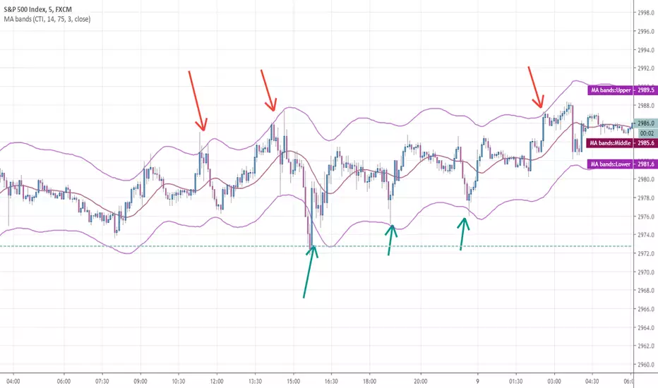
Any MA bands (TMA bands V2)Hi everyone
Website will be opening very shortly :) Sorting out the last details and we're so excited to finally roll-out our different Algorithm Builders for you guys
Forewords
This present script is an evolution of the TMA bands . I would never have expected that script to become so popular to be honest
This is not only a study or idea but a really proven method and I'm glad that many of you are using it already. But please, whenever you see a new script out there, even if it looks cool and promising, please test it on a demo account for a week or on a LIVE account but with tiny amounts every time.
Many times, what you see on the chart is not what will happen in reality. I know that most of you will agree and I know exactly why we see this behavior... I'll give more details in a later post
I have plenty of methods like that one and I'll detail them on my website (and a bit on TradingView) starting next month
TMA bands on steroids
Someone asked me privately to make a generic version of the TMA bands and make it compatible with other standards Moving Average types. That's it for the specifications really as I didn't do much than re-using some piece of my own code
Suggested (but not mandatory) methodology
1) The Take Profit 1 is the middle line, Take Profit 2 is the opposite band.
2) Once the TP1 is hit, set your Stop Loss to breakeven
3) Once the TP2 is hit, if you still want to stay in the trade, set your Stop Loss to the TP1
It will be a powerful tool in your arsenal for some scalp/intraday trades
Wishing you all of you a great and profitable day
PS
It's strictly forbidden to republish this script without my explicit approval. All my posts are copyrighted from now on
Obviously you can use but not republish and get the credit or even worse... some money from your own clients
Dave
____________________________________________________________
Be sure to hit the thumbs up. Building those indicators take a lot of time and likes are always rewarding for me :) (tips are accepted too)
- If you want to suggest some indicators that I can develop and share with the community, please use my personal TRELLO board
- I'm an officially approved PineEditor/LUA/MT4 approved mentor on codementor. You can request a coaching with me if you want and I'll teach you how to build kick-ass indicators and strategies
Jump on a 1 to 1 coaching with me
- You can also hire for a custom dev of your indicator/strategy/bot/chrome extension/python
Disclaimer:
Trading involves a high level of financial risk, and may not be appropriate because you may experience losses greater than your deposit. Leverage can be against you.
Do not trade with capital that you can not afford to lose. You must be aware and have a complete understanding of all the risks associated with the market and trading. We can not be held responsible for any loss you incur.
Trading also involves risks of gambling addiction.
Please notice I do not provide financial advice - my indicators, strategies, educational ideas are intended to provide only some source code for anyone interested in improving their trading
The proprietary indicators and strategies developed by Best Trading Indicator, the object of intellectual property rights are and remain the exclusive property of Best Trading Indicator, at the exclusion of images and videos and texts free of rights or provided by the Company or external legal or physical person.
No assignment of intellectual property rights is carried out through these Terms and Conditions.
Any total or partial reproduction, modification or use of these properties for any reason whatsoever is strictly prohibited without the express written authorization of the Company.
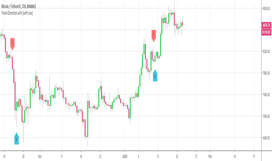
Customizable Trend Direction (Open-Source)Hello everyone
I received a ton of requests for this script so I decided to share it
I did it for a client who didn't want to pay (you can all blame... or even thank him for this script) in the end and I don't want to sell it on my website.
Not because it's not interesting but because my website will be a place to showcase and rent the Algorithm Builders mostly
What is it about?
Basically, it shows how you could convert a plotshape into a label.new object. Very interesting if you want someday to convert your V3 script into V4
With this script, it shows that you can in V4 ( but couldn't do in V3 ) do the followings :
- change dynamically the size (from tiny to huge) of any object
- change dynamically the text (from whatever to whatever) of any object
Screenshot of the user interface
imgur.com
Other use cases
I did it with the Trend Direction but could work with anything really.
- Any indicator with a visual signal. You can know personalized from a user interface the text, size and also the vertical shift. I didn't do it for that one but label.new takes a (x,y) coordinates so playing with y is fairly easy to achieve a dynamic vertical shift
- Even with this script Plotchar-How-to-draw-external-symbols-on-a-chart/ but would require to be updated with a label.new object and with a shape.none parameter so that we'll only see the icon/symbol displayed
- The colors also can be change dynamically using presets Presets-Selector-FRIDAY-NIGHT-CHALLENGE/ . If you have an indicator showing a BULLISH and a BEARISH signal, then you could, for instance, configure colors presets according to the timeframe of the chart or the indicator input, etc (sky is the limit ^^)
Be sure to hit the thumbs up at it motivates me to research what Pinescript can offer and share with the community
Dave
____________________________________________________________
- I'm an officially approved PineEditor/LUA/MT4 approved mentor on codementor. You can request a coaching with me if you want and I'll teach you how to build kick-ass indicators and strategies
Jump on a 1 to 1 coaching with me
- You can also hire for a custom dev of your indicator/strategy/bot/chrome extension/python
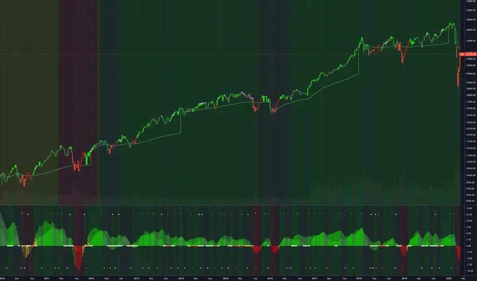
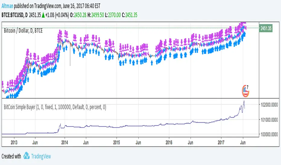
BitCoin Simple BuyerMany people asking me: How to find the right time to exit BitCoin long position? First, that comes to mind is Do Not use simple Buy-and-Hold strategy, but make short-term trades. Here is the simple algorithm for D1 or 4H timeframes.
OrangePulse v3.0 Lite - Educational DCA StrategyThis open-source script is a simplified version of the OrangePulse algorithm, designed for educational purposes to demonstrate the power of Dollar Cost Averaging (DCA) and Mean Reversion.
📈 Strategy Logic:
The script uses a combination of Bollinger Bands and RSI (Relative Strength Index) to identify potential mean reversion opportunities.
- Entry: Triggered when price pushes below the lower Bollinger Band while RSI is in oversold territory.
- Management: Utilizes up to 3 Safety Orders (DCA) to improve the average entry price during pullbacks.
🎯 Features:
• Customizable Volume Scale and Step Scale for Safety Orders.
• Visual AVG price line and TP/SL levels.
• Time-window filter for backtesting.
• Real-time Status Table for position monitoring.
This script is shared in the spirit of open-source development on TradingView. It is intended to help traders understand how automated position building and risk management work in volatile markets.
Check my profile status/bio for more information on our project.
⚠️ Disclaimer: For educational purposes only. Past performance does not guarantee future results.

BNF (Kotegawa) Strategy [CB Algos]STRATEGY: BNF (Kotegawa) Mean Reversion Strategy
DEVELOPED BY: CB Algos
DESCRIPTION:
This indicator replicates the trading style of Takashi Kotegawa (BNF).
It calculates the percentage deviation of the price from the 25-period SMA.
HOW TO USE:
1. Look for 'Lime' bars (Extreme Buy) or 'Teal' bars (Moderate Buy). These indicate the price has dropped significantly below the average.
2. Look for 'Red' bars (Extreme Sell) as profit-taking zones.
3. Use the Info Panel to see the exact current deviation %.

Volume Anomaly Reversal DetectionVolume Anomaly Reversal Detection (VARD System)
🎯 What This Indicator Does
This indicator identifies potential trend reversals by detecting abnormal volume activity that often precedes significant price movements. It combines volume anomaly detection with dynamic trend analysis to generate actionable BUY/SELL signals.
📊 Core Concept & Methodology
Volume Anomaly Detection
The indicator analyzes directional volume (buying vs selling pressure) from a lower timeframe and calculates Z-scores to identify statistically significant volume spikes.
Z-Score Formula:
Z = (Current Volume - Average Volume) / Standard Deviation
When volume exceeds the threshold (default: 3 standard deviations above mean), it signals unusual market activity - often caused by forced liquidations or capitulation.
Dynamic Trend Filter
A custom trend-following algorithm based on ATR (Average True Range) bands determines the current market direction:
Price above lower band = Uptrend
Price below upper band = Downtrend
Signal Logic
Volume anomaly detected during an existing trend
Trend reversal confirmed within the confirmation window
Signal generated = BUY or SELL label appears
⚙️ Settings Explained
SettingDefaultDescriptionAnalysis Timeframe15minLower timeframe for volume samplingStatistical Lookback200Bars used for Z-score calculationAnomaly Sensitivity3.0Z-score threshold (lower = more signals)Confirmation Window50Max bars between anomaly and trend flipATR Multiplier2.0Trend band widthTrend Period10ATR calculation length
📖 How To Use
Entry Signals
BUY: Green label appears below bar - consider long positions
SELL: Red label appears above bar - consider short positions
Volume Anomaly Markers (⬥)
Small diamonds indicate detected volume spikes
These are early warnings before confirmed signals
Useful for anticipating potential reversals
Trend Bands
Colored zones show active signal direction
Stay with the trend until opposite signal appears
Best Practices
Confirm with price action - Look for support/resistance levels
Use appropriate timeframes - Works on all timeframes, but 1H-4H recommended
Manage risk - Always use stop losses
Avoid ranging markets - Best in trending/volatile conditions
⚠️ Important Notes
No indicator is perfect - Use as part of a complete trading strategy
Volume data required - Will show warning if volume unavailable
Not financial advice - Always do your own research
🔔 Alerts Available
BUY Signal Confirmed
SELL Signal Confirmed
Volume Anomaly (Buy Setup)
Volume Anomaly (Sell Setup)

Miela Labs | John Dee's Watchtower [257-463]Bridging the gap between 16th-century esoteric mathematics and modern algorithmic trading.
The Enochian Watchtower is not merely a trend indicator; it is a computational artifact developed by Miela Labs LLC. This script translates Dr. John Dee’s "Great Table of the Watchtowers" and the "Sigil Dei Aemeth" into actionable financial data points.
Using our proprietary Occultator V2.0 Engine, we have derived specific mathematical constants that resonate with the current market structure.
🏛️ The Algorithmic Logic
This indicator utilizes three sacred numbers to construct a "Future Vision" of the market:
1. The Axis Mundi (Vector 257): derived from Fermat Primes and John Dee’s Grid coordinates. This Weighted Moving Average (WMA) acts as the spinal cord of the trend.
2. The Gates (Cipher 463): A prime number derived from the "Galethog" cipher stride. These bands define the absolute volatility limits (Heaven & Earth Gates).
3. Future Vision (Offset 21): Utilizing Fibonacci time sequences, the indicator projects Support and Resistance levels 21 bars into the future, allowing traders to anticipate market movements before they occur.
⚡ How to Use
• The Trend: If price is above the Purple Axis (257), the market is in a bullish phase.
• The Entry: Look for "L" (Long) and "S" (Short) signals. These are confirmed when the signal path crosses the Axis.
• The Future: Watch the projected lines on the right side of the chart to identify upcoming resistance zones.
About Miela Labs
Miela Labs is a Technomancy Research Institute based in McKinney, Texas. We specialize in building open-source esoteric trading tools and the Magic Programming Language (MPL).
🌐 Official Hub: Visit Miela Labs
💻 Source Code & Research: GitHub Repository
Disclaimer: This tool is for educational and research purposes only. It demonstrates the application of esoteric mathematics in financial analysis. Trade responsibly.

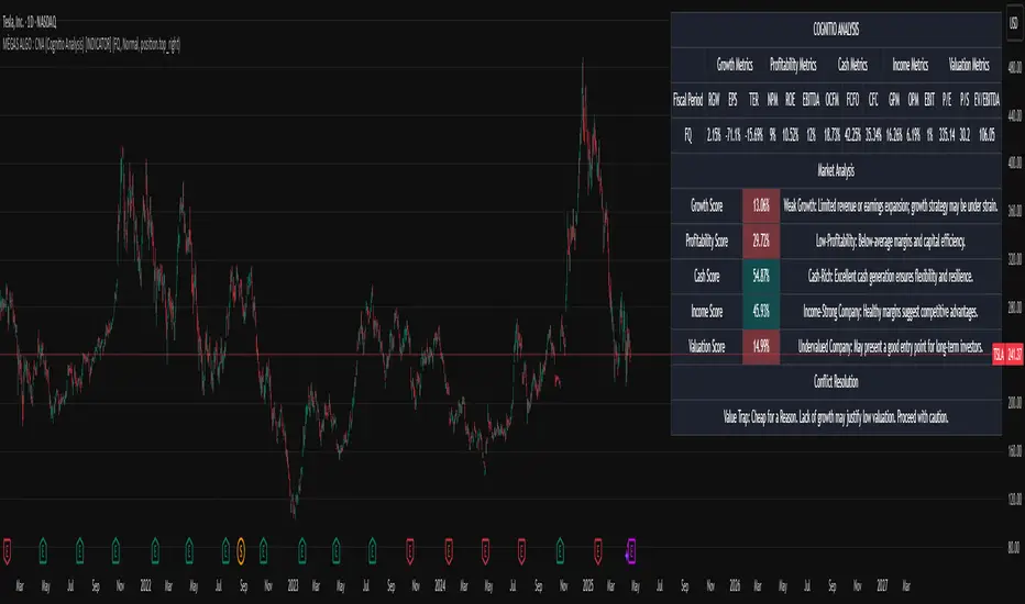
MÈGAS ALGO : CNA (Cognitio Analysis) [INDICATOR]Overview
The CNA (Cognitio Analysis) is a comprehensive financial analysis tool designed to evaluate the overall health and potential of a market or company based on fundamental metrics. It aggregates data across five key metric groups—**Growth**, **Profitability**, **Cash Flow**, **Income**, and **Valuation**—to provide a final interpretation of market conditions. The indicator dynamically adapts to the selected fiscal period (Quarter, Year, or Trailing Twelve Months) and delivers insights into dominant trends and conflicting signals.
Key Features
1. Customizable Fiscal Period:
- Users can select between "Quarter", "Year", or "Trailing Twelve Months" (TTM) to analyze data for their desired timeframe.
2. Dynamic Table Visualization:
- Displays raw metric values, aggregated scores, and the final interpretation in an intuitive
table.
- Highlights the final interpretation with dynamic background colors (`color.teal` for bullish,
`color.red` for bearish, etc.).
3. Comprehensive Data Integration:
- Pulls financial data using TradingView's `request.financial()` function for metrics like
revenue, earnings, margins, and valuation ratios.
4. Normalization and Scoring:
- Normalizes data to create a consistent scoring system, ensuring accurate comparisons across
metrics.
How It Works
1. Metric Group Analysis
- Growth Metrics: Measures revenue growth, earnings per share (EPS) growth, and tax
efficiency.
- Profitability Metrics: Analyzes net profit margin, return on equity (ROE), and EBITDA margin.
- Cash Metrics: Assesses operating cash flow margin, free cash flow to operating cash flow
ratio, and cash flow coverage.
- Income Metrics: Examines gross profit margin, operating profit margin, and EBIT margin.
- Valuation Metrics: Evaluates price-to-earnings (P/E), price-to-sales (P/S), and enterprise
value-to-EBITDA (EV/EBITDA).
2. Dynamic Scoring System
- Metrics are normalized to ensure consistency across different scales.
- A geometric mean is used to calculate scores for each metric group, ensuring that all metrics
within a group contribute equally to the final score.
3. Dominant Trend Identification
- Scores from all five metric groups are aggregated to determine the **dominant trend** of the
market.
- The dominant trend is categorized as:
- Bullish: Strong fundamentals across most metrics.
- Bearish: Weak fundamentals across most metrics.
- Neutral: Balanced conditions with no clear direction.
- Unclear: Mixed signals dominate, requiring further monitoring.
4. Conflicting Signals Interpretation
- The indicator identifies scenarios where metrics conflict (e.g., high growth but low valuation).
- These conflicting signals provide nuanced insights into market conditions, highlighting rare opportunities or potential risks.
How to Use the Indicator
1. Select Fiscal Period:
- Choose between "FQ", "FY", or "TTM" to analyze data for the desired timeframe.
2. Review Metric Scores:
- Examine the scores for each metric group (Growth, Profitability, Cash, Income, Valuation) to
understand the underlying performance.
3. Interpret Final Output:
- The final interpretation provides a summary of the dominant trend and conflicting signals,
helping users make informed decisions.
4. Dynamic Coloring:
- Use the dynamic background colors in the table to quickly identify market sentiment
(bullish, bearish, neutral, or mixed).
Applications
- Identifying Opportunities:
- Look for bullish dominant trends combined with undervalued growth opportunities for
potential long positions.
- Avoiding Risks:
- Watch out for bearish dominant trends with overvaluation alerts to avoid potential losses.
- Monitoring Neutral Markets:
- Use the indicator to identify neutral markets and wait for clearer signals before making
decisions.
Conclusion
The CNA (Cognitio Analysis) is a powerful tool for traders and investors seeking to make informed decisions based on fundamental analysis. By combining detailed metric evaluations, dynamic scoring, and sentiment-based interpretations, this indicator provides a comprehensive view of market conditions. Whether you're identifying undervalued opportunities, avoiding overvalued risks, or monitoring neutral markets, this indicator equips you with the insights needed to navigate complex financial landscapes.
Please Note:
This indicator is provided for informational and educational purposes only. It is not financial advice, and it should not be considered a recommendation to buy, sell, or trade any financial instrument. Trading involves significant risks, including the potential loss of your entire investment. Always conduct your own research and consult with a licensed financial advisor before making any trading decisions.
The results and images provided are based on algorithms and historical/paid real-time market data but do not guarantee future results or accuracy. Use this tool at your own risk, and understand that past performance is not indicative of future outc
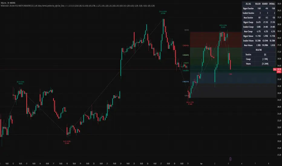
MÈGAS ALGO : ZIG-ZAG CYCLE INSIGTH [INDICATOR]Overview
The Zig-Zag Cycle Insigth is a revisited version of the classic Zig Zag indicator, designed to provide traders with a more comprehensive and actionable view of price movements.
This advanced tool not only highlights significant price swings but also incorporates additional features such as cycle analysis, real-time data tracking, and Fibonacci retracement levels. These enhancements make it an invaluable resource for identifying trends, potential reversal points, and market structure.
This indicator adheres to TradingView's guidelines and is optimized for both technical analysts and active traders who seek deeper insights into market dynamics.
Key Features:
1. Customizable Thresholds for Price Movements:
- Users can set personalized thresholds for price movement percentages and time periods.
This ensures that only significant price swings are plotted, reducing noise and increasing
clarity.
- Straight lines connect swing highs and lows, providing a cleaner visual representation of
the trend.
2. Cycle Analysis Table:
- A dynamic table is included to analyze price cycles based on three key factors:
- Price Change: Measures the magnitude of each swing (high-to-low or low-to-high).
- Time Duration (Bar Count): Tracks the number of bars elapsed between consecutive swings,
offering precise timing insights.
- Volume: Analyzes trading volume during each segment of the cycle.
- The indicator calculates the **maximum**, **minimum**, and **mean** values for each
parameter across all completed cycles, providing deeper statistical insights into market
behavior.
- This table updates in real-time, offering traders a quantitative understanding of how price
behaves over different cycles.
3. Real-Time Data Integration:
- The indicator displays live updates of current price action relative to the last identified
swing high/low. This includes:
- Current distance from the last pivot point.
- Percentage change since the last pivot.
- Volume traded since the last pivot.
4. Fibonacci Retracement Levels:
- Integrated Fibonacci retracement levels are dynamically calculated based on the most
recent significant swing high and low.
- Key retracement levels (23.6%, 38.2%, 50%, 61.8%, and 78.6%) are plotted alongside the Zig
Zag lines, helping traders identify potential support/resistance zones.
- Extension levels (100%, 161.8%, etc.) are also included to anticipate possible breakout
targets.
5. Customizable Alerts:
- Users can configure alerts for specific real-time conditions, such as:
- Price Change
- Duration
- Volume
- Fibonacci Retracement Levels
How It Works:
1. Zig Zag Identification:
- The indicator scans historical price data to identify significant turning points where the
price moves by at least the user-defined percentage threshold.
- These turning points are connected by straight lines to form the Zig Zag pattern.
2. Cycle Analysis:
For each completed cycle (from one swing high/low to the next), the indicator calculates:
- Price Change: Difference between the start and end prices of the cycle.
- Maximum Price Change: The largest price difference observed across all cycles.
- Minimum Price Change: The smallest price difference observed across all cycles.
- Mean Price Change: The average price difference across all cycles.
- Time Duration (Bar Count): Number of bars elapsed between consecutive swings.
- Maximum Duration: The longest cycle in terms of bar count.
- Minimum Duration: The shortest cycle in terms of bar count.
- Mean Duration: The average cycle length in terms of bar count.
- Volume: Total volume traded during the cycle.
- Maximum Volume: The highest volume traded during any single cycle.
- Minimum Volume: The lowest volume traded during any single cycle.
- Mean Volume: The average volume traded across all cycles.
- These calculations provide traders with a statistical overview of market behavior, enabling
them to identify patterns and anomalies in price, time, and volume.
3. Fibonacci Integration:
- Once a new swing high or low is identified, the indicator automatically calculates Fibonacci
retracement and extension levels.
- These levels serve as reference points for potential entry/exit opportunities.
4. Real-Time Updates:
- As the market evolves, the indicator continuously monitors the relationship between the
current price and the last identified swing point.
- Real-time metrics, such as percentage change and volume, are updated dynamically.
5. Alerts Based on Real-Time Parameters:
- The indicator allows users to set customizable alerts based on real-time conditions:
- Price Change Alert: Triggered when the real-time price change is less or greater than a
predefined percentage threshold (e.g., > or < fixed value).
- Duration Alert: Triggered when the cycle duration (in bars) is less or greater than a
predefined
bar count threshold (e.g., > or < fixed value).
- Volume Alert: Triggered when the trading volume during the current cycle is less or greater
than a predefined volume threshold (e.g., > or < fixed value).
Advantages of Zig-Zag Cycle Insigth
- Comprehensive Insights: Combining cycle analysis, Fibonacci retracements, and real-time data
provides a holistic view of market conditions.
- Statistical Analysis: The inclusion of maximum, minimum, and mean values for price change,
duration, and volume offers deeper insights into market behavior.
- Actionable Signals: Customizable alerts ensure traders never miss critical market events based
on real-time price, duration, and volume parameters.
- User-Friendly Design: Clear visuals and intuitive controls make it accessible for traders of all
skill levels.
Reference:
TradingView/ZigZag
TradingView/AutofibRetracement
Please Note:
This indicator is provided for informational and educational purposes only. It is not financial advice, and it should not be considered a recommendation to buy, sell, or trade any financial instrument. Trading involves significant risks, including the potential loss of your entire investment. Always conduct your own research and consult with a licensed financial advisor before making any trading decisions.
The results and images provided are based on algorithms and historical/paid real-time market data but do not guarantee future results or accuracy. Use this tool at your own risk, and understand that past performance is not indicative of future outcomes.
Market Structure Algo V2 [OmegaTools]The Market Structure Algo V2 (MS Algo V2) is an advanced TradingView indicator developed by OmegaTools to provide traders with a comprehensive analysis of market structure. This tool refines the insights provided by its predecessor, combining enhanced pivot point analysis, dynamic market structure scoring, and zone visualization to deliver an intuitive view of potential market movements. Through custom settings, the MS Algo V2 allows users to tailor the indicator to fit their trading strategies more closely, offering enhanced adaptability to both short-term and long-term trends.
Core Functionality
The MS Algo V2 differentiates between internal and external market structures by analyzing pivot highs and lows over user-defined periods. The internal market structure focuses on shorter timeframes, providing insights into recent price action, while the external structure considers broader trends. This dual-layered approach helps traders distinguish between immediate and overarching market trends.
The indicator introduces improved visualization for areas of interest or zones around pivot points, adjustable through zone distance settings. These zones serve as potential support and resistance areas, helping traders anticipate price reactions at key levels. In addition to the zones, the indicator now provides gradient-based color coding on bars, reflecting the market structure’s bullish or bearish intensity. This visual enhancement aids in quickly interpreting the current trend's strength.
Dynamic signal generation has been refined in MS Algo V2. The indicator now offers both classic signals and breakout signals based on the market structure, including entries, exits, and change-of-character (CHoCH) alerts. Signals are generated based on price interactions with pivot levels, indicating potential long and short opportunities.
Operational Mechanism
The MS Algo V2 calculates pivot highs and lows over specified periods to define internal and external market structures. A market structure score is derived from these pivot points, classifying the market into bullish or bearish extremes. Signals are generated as the closing price interacts with these levels, marking entry and exit points based on the calculated structure.
A new feature in this version is zone visualization, where zones are plotted around a dynamic moving average derived from the exponential and simple moving averages (EMA and SMA). The zones are adjusted based on ATR (Average True Range) and the specified zone distance percentile, providing a clear visual representation of potential support and resistance regions. The external and internal zones are represented with different levels of transparency for quick reference.
Usage Guidelines
To apply the MS Algo V2 to your TradingView charts, adjust the internal and external market structure settings to match your preferred analysis timeframes. The line style and width of each structure can also be customized for a tailored view. The Zone Distance setting allows users to define the percentile range of the zones around the moving average, providing further flexibility in identifying potential areas of support and resistance.
For a color-coded overview of market sentiment, the bar gradient feature can be enabled. This option uses a gradient that reflects the bullish or bearish intensity of the market structure, giving traders a visual cue on the market’s overall trend. Color-coded signals and zone fill areas further assist in interpreting the current market structure and identifying potential trade areas.
The indicator includes customizable alerts for long and short signals, as well as specific breakout alerts (BOS) and change-of-character (CHoCH) signals. These alerts can help traders stay informed about significant market structure changes, supporting timely trading decisions.
Understanding the Indicator’s Originality
The MS Algo V2 stands out due to its robust integration of pivot analysis, zone visualization, and market structure scoring, offering a unique perspective on market dynamics. With features like color-coded signals, bar gradients, and configurable alerts, MS Algo V2 provides an edge in understanding both the current market environment and potential turning points. This indicator’s ability to represent the market’s structure visually makes it a powerful addition to any trader’s toolkit, especially for those seeking a deeper, multi-layered approach to market analysis.

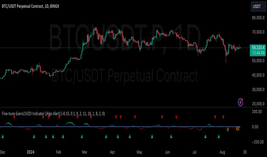
GannLSVZO Indicator [Algo Alert]The Volume Zone oscillator breaks up volume activity into positive and negative categories. It is positive when the current closing price is greater than the prior closing price and negative when it's lower than the prior closing price. The resulting curve plots through relative percentage levels that yield a series of buy and sell signals, depending on level and indicator direction.
The Gann Laplace Smoothed Volume Zone Oscillator GannLSVZO is a refined version of the Volume Zone Oscillator, enhanced by the implementation of the upgraded Discrete Fourier Transform, the Laplace Stieltjes Transform. Its primary function is to streamline price data and diminish market noise, thus offering a clearer and more precise reflection of price trends.
By combining the Laplace with Gann Swing Entries and Exits (orange X) and with Ehler's white noise histogram, users gain a comprehensive perspective on volume-related market conditions.
HOW TO USE THE INDICATOR:
The default period is 2 but can be adjusted after backtesting. (I suggest 5 VZO length and NoiceR max length 8 as-well)
The VZO points to a positive trend when it is rising above the 0% level, and a negative trend when it is falling below the 0% level. 0% level can be adjusted in setting by adjusting VzoDifference. Oscillations rising below 0% level or falling above 0% level result in a natural trend.
ORIGINALITY & USFULLNESS:
Personal combination of Gann swings and Laplace Stieltjes Transform of a price which results in less noise Volume Zone Oscillator.
The Laplace Stieltjes Transform is a mathematical technique that transforms discrete data from the time domain into its corresponding representation in the frequency domain. This process involves breaking down a signal into its individual frequency components, thereby exposing the amplitude and phase characteristics inherent in each frequency element.
This indicator utilizes the concept of Ehler's Universal Oscillator and displays a histogram, offering critical insights into the prevailing levels of market noise. The Ehler's Universal Oscillator is grounded in a statistical model that captures the erratic and unpredictable nature of market movements. Through the application of this principle, the histogram aids traders in pinpointing times when market volatility is either rising or subsiding.
The Gann swings and the Gan swing strategy is developed by meomeo105, this Gann high and low algorithm forms the basis of the EMA modification.
DETAILED DESCRIPTION:
My detailed description of the indicator and use cases which I find very valuable.
What is oscillator?
Oscillators are chart indicators that can assist a trader in determining overbought or oversold conditions in ranging (non-trending) markets.
What is volume zone oscillator?
Price Zone Oscillator measures if the most recent closing price is above or below the preceding closing price.
Volume Zone Oscillator is Volume multiplied by the 1 or -1 depending on the difference of the preceding 2 close prices and smoothed with Exponential moving Average.
What does this mean?
If the VZO is above 0 and VZO is rising. We have a bullish trend. Most likely.
If the VZO is below 0 and VZO is falling. We have a bearish trend. Most likely.
Rising means that VZO on close is higher than the previous day.
Falling means that VZO on close is lower than the previous day.
What if VZO is falling above 0 line?
It means we have a high probability of a bearish trend.
Thus the indicator returns 0 and Strategy closes all it's positions when falling above 0 (or rising bellow 0) and we combine higher and lower timeframes to gauge the trend.
What is approximation and smoothing?
They are mathematical concepts for making a discrete set of numbers a
continuous curved line.
Laplace Stieltjes Transform approximation of a close price are taken from aprox library.
Key Features:
You can tailor the Indicator/Strategy to your preferences with adjustable parameters such as VZO length, noise reduction settings, and smoothing length.
Volume Zone Oscillator (VZO) shows market sentiment with the VZO, enhanced with Exponential Moving Average (EMA) smoothing for clearer trend identification.
Noise Reduction leverages Euler's White noise capabilities for effective noise reduction in the VZO, providing a cleaner and more accurate representation of market dynamics.
Choose between the traditional Fast Laplace Stieltjes Transform (FLT) and the innovative Double Discrete Fourier Transform (DTF32) soothed price series to suit your analytical needs.
Use dynamic calculation of Laplace coefficient or the static one. You may modify those inputs and Strategy entries with Gann swings.
I suggest using "Close all" input False when fine-tuning Inputs for 1 TimeFrame. When you export data to Excel/Numbers/GSheets I suggest using "Close all" input as True, except for the lowest TimeFrame. I suggest using 100% equity as your default quantity for fine-tune purposes. I have to mention that 100% equity may lead to unrealistic backtesting results. Be avare. When backtesting for trading purposes use Contracts or USDT.
DeQuex Algo BISTIntroduction:
The DeQuex Algo is an advanced technical analysis tool designed to help traders identify high-probability entry and exit points in the Borsa Istanbul (BIST) market. This updated version incorporates an adaptive MACD to reduce false signals and improve the overall reliability of the indicator.
Key Features:
1. Adaptive MACD: The script utilizes an adaptive MACD that dynamically adjusts to market volatility, reducing the occurrence of false signals often associated with traditional MACD implementations.
2. RSI Confirmation: In addition to the adaptive MACD, the DeQuex Algo also considers RSI readings to provide stronger confirmation for buy and sell signals.
3. Signal Types:
- Buy Signal: Triggered when the adaptive MACD crosses above its signal line.
- Sell Signal: Triggered when the adaptive MACD crosses below its signal line.
- Strong Buy Signal: Triggered when both the adaptive MACD and RSI cross above their respective thresholds, indicating a high-probability bullish setup.
- Strong Sell Signal: Triggered when both the adaptive MACD and RSI cross below their respective thresholds, indicating a high-probability bearish setup.
4. Price Bar Highlighting: The script color-codes price bars to provide a visual representation of the current trend. Green bars indicate an uptrend, red bars indicate a downtrend, and purple bars signify a period of consolidation or uncertainty. This feature allows traders to quickly assess the market context at a glance.
5. Customizable Alerts: Users can enable alerts for each signal type, ensuring they never miss a potential trading opportunity.
6. Dynamic Support and Resistance: The DeQuex Algo incorporates dynamic support and resistance levels based on market volatility. These levels are plotted using an innovative approach that combines Donchian channels with a Kalman filter for smoother, more reliable zones.
7. User-Friendly Inputs: The script provides a range of input parameters, allowing traders to fine-tune the indicator's sensitivity and adapt it to their preferred trading style and timeframe.
How to Use:
1. Add the DeQuex Algo indicator to your TradingView chart.
2. Customize the input parameters as desired, or use the default settings.
3. Enable alerts for your preferred signal types.
4. Look for buy and sell signals based on the adaptive MACD and RSI readings, paying attention to the color-coded price bars for additional context.
5. Consider the dynamic support and resistance levels when planning your entries, exits, and stop-loss placements.
Please note that while the DeQuex Algo is designed to identify high-probability setups, no indicator is perfect, and false signals may still occur. Always use proper risk management and consider other factors, such as market sentiment and fundamental analysis, when making trading decisions.
We hope that the DeQuex Algo will be a valuable addition to your trading toolbox, and we welcome any feedback or suggestions for further improvement.
Best regards,
BrandonJames1337
TR:
İşte güncellenmiş DeQuex Algo göstergeniz için önerilen bir açıklama:
Giriş:
DeQuex Algo, yatırımcıların Borsa İstanbul (BIST) piyasasında yüksek olasılıklı giriş ve çıkış noktalarını belirlemelerine yardımcı olmak için tasarlanmış gelişmiş bir teknik analiz aracıdır. Bu güncellenmiş sürüm, yanlış sinyalleri azaltmak ve göstergenin genel güvenilirliğini artırmak için uyarlanabilir bir MACD içerir.
Temel Özellikler:
1. Uyarlanabilir MACD: Komut dosyası, piyasa oynaklığına dinamik olarak ayarlanan ve genellikle geleneksel MACD uygulamalarıyla ilişkili yanlış sinyallerin oluşumunu azaltan uyarlanabilir bir MACD kullanır.
2. RSI Onayı: Uyarlanabilir MACD'ye ek olarak DeQuex Algo, alım ve satım sinyalleri için daha güçlü onay sağlamak üzere RSI okumalarını da dikkate alır.
3. Sinyal Türleri:
- Alış Sinyali: Uyarlanabilir MACD sinyal çizgisinin üzerine çıktığında tetiklenir.
- Satış Sinyali: Uyarlanabilir MACD sinyal çizgisinin altından geçtiğinde tetiklenir.
- Güçlü Alış Sinyali: Hem uyarlanabilir MACD hem de RSI kendi eşiklerinin üzerine çıktığında tetiklenir ve yüksek olasılıklı bir yükseliş düzenine işaret eder.
- Güçlü Satış Sinyali: Hem uyarlanabilir MACD hem de RSI kendi eşiklerinin altına düştüğünde tetiklenir ve yüksek olasılıklı bir düşüş düzenine işaret eder.
4. Fiyat Çubuğu Vurgulama: Komut dosyası, mevcut eğilimin görsel bir temsilini sağlamak için fiyat çubuklarını renk kodlarıyla kodlar. Yeşil çubuklar yükseliş trendini, kırmızı çubuklar düşüş trendini ve mor çubuklar ise konsolidasyon veya belirsizlik dönemini gösterir. Bu özellik, yatırımcıların piyasa bağlamını bir bakışta hızlı bir şekilde değerlendirmelerine olanak tanır.
5. Özelleştirilebilir Uyarılar: Kullanıcılar her sinyal türü için uyarıları etkinleştirerek potansiyel bir alım satım fırsatını asla kaçırmamalarını sağlayabilir.
6. Dinamik Destek ve Direnç: DeQuex Algo, piyasa oynaklığına dayalı dinamik destek ve direnç seviyeleri içerir. Bu seviyeler, daha yumuşak ve daha güvenilir bölgeler için Donchian kanallarını Kalman filtresiyle birleştiren yenilikçi bir yaklaşım kullanılarak çizilir.
7. Kullanıcı Dostu Girişler: Komut dosyası, yatırımcıların göstergenin hassasiyetini ince ayarlamalarına ve tercih ettikleri ticaret tarzına ve zaman dilimine uyarlamalarına olanak tanıyan bir dizi giriş parametresi sağlar.
Nasıl Kullanılır:
1. DeQuex Algo göstergesini TradingView grafiğinize ekleyin.
2. Giriş parametrelerini istediğiniz gibi özelleştirin veya varsayılan ayarları kullanın.
3. Tercih ettiğiniz sinyal türleri için uyarıları etkinleştirin.
4. Ek bağlam için renk kodlu fiyat çubuklarına dikkat ederek uyarlanabilir MACD ve RSI okumalarına dayalı alım ve satım sinyallerini arayın.
5. Girişlerinizi, çıkışlarınızı ve stop-loss yerleşimlerinizi planlarken dinamik destek ve direnç seviyelerini göz önünde bulundurun.
DeQuex Algo yüksek olasılıklı kurulumları belirlemek için tasarlanmış olsa da, hiçbir göstergenin mükemmel olmadığını ve yine de yanlış sinyallerin oluşabileceğini lütfen unutmayın. Alım satım kararları verirken her zaman uygun risk yönetimini kullanın ve piyasa duyarlılığı ve temel analiz gibi diğer faktörleri göz önünde bulundurun.
DeQuex Algo'nun ticaret araç kutunuza değerli bir katkı sağlayacağını umuyor ve daha fazla iyileştirme için her türlü geri bildirim veya öneriyi memnuniyetle karşılıyoruz.
Saygılarımla,
BrandonJames1337

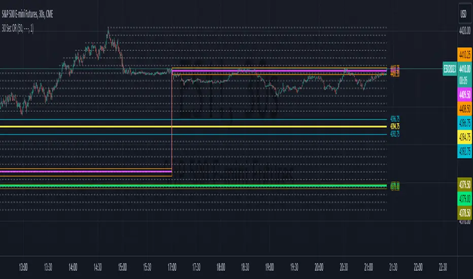
30 Second Futures Session Open RangeThis indicator displays 30 second opening ranges from Globex, Europe, and RTH sessions.
From the RTH session range, it also displays infinitely generating Price Targets based on a % of the opening range size.
I am retrieving the 30 second data using the new "request.security_lower_tf()" function.
The importance of these levels is based on the idea that when the market opens, algorithms establish their positions within the first 30 seconds.
These areas can also be seen as potential areas of support and resistance throughout the sessions.
Enjoy!
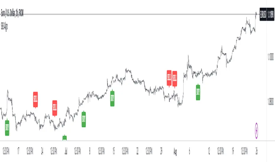
SBS AlgoHello traders, I am here again with a new and improved indicator.
This indicator is based on a pivot breakout algorithm which gives buy and sell signals according to the breakout of trendline. This is an advanced version of another script. It also takes price action into consideration along with some basic indicators like MACD and ADX to give good entry signals.
NOTE: This indicator is not designed to take entries completely based on signals it gives. Please use it along with your trading strategy to add more confluence to your trading system and maximize your profits.
I hope you guys will like this one too .Enjoy 👍
In case you find any bug, please do report in comment section .Thank you.
BollingerBands Strat + pending order alerts via TradingConnectorSoftware part of algotrading is simpler than you think. TradingView is a great place to do this actually. To present it, I'm publishing each of the default strategies you can find in Pinescript editor's "built-in" list with slight modification - I'm only adding 2 lines of code, which will trigger alerts, ready to be forwarded to your broker via TradingConnector and instantly executed there. Alerts added in this script: 14, 17, 20 and 23.
SCRIPT INCLUDES PENDING ORDERS AND ALERTS! Alert will be sent to MetaTrader when order is triggered, but not yet filled. That means if market conditions change and order does not get filled, it needs to be cancelled as well, and there are alerts for that in the script as well.
How it works:
1. TradingView alert fires.
2. TradingConnector catches it and forwards to MetaTrader4/5 you got from your broker.
3. Trade gets executed inside MetaTrader within 1 second of fired alert.
When configuring alert, make sure to select "alert() function calls only" in CreateAlert popup. One alert per ticker is required.
Adding stop-loss, take-profit, trailing-stop, break-even or executing pending orders is also possible. These topics have been covered in other example posts.
This routing works for Forex, indices, stocks, crypto - anything your broker offers via their MetaTrader4 or 5.
Disclaimer: This concept is presented for educational purposes only. Profitable results of trading this strategy are not guaranteed even if the backtest suggests so. By no means this post can be considered a trading advice. You trade at your own risk.
If you are thinking to execute this particular strategy, make sure to find the instrument, settings and timeframe which you like most. You can do this by your own research only.

Consecutive Up/Down Strat + alerts via TradingConnector to ForexSoftware part of algotrading is simpler than you think. TradingView is a great place to do this actually. To present it, I'm publishing each of the default strategies you can find in Pinescript editor's "built-in" list with slight modification - I'm only adding 2 lines of code, which will trigger alerts, ready to be forwarded to your broker via TradingConnector and instantly executed there. Alerts added in this script: 12 and 15.
How it works:
1. TradingView alert fires.
2. TradingConnector catches it and forwards to MetaTrader4/5 you got from your broker.
3. Trade gets executed inside MetaTrader within 1 second of fired alert.
When configuring alert, make sure to select "alert() function calls only" in CreateAlert popup. One alert per ticker is required.
Adding stop-loss, take-profit, trailing-stop, break-even or executing pending orders is also possible. These topics have been covered in other example posts.
This routing works for Forex, indices, stocks, crypto - anything your broker offers via their MetaTrader4 or 5.
Disclaimer: This concept is presented for educational purposes only. Profitable results of trading this strategy are not guaranteed even if the backtest suggests so. By no means this post can be considered a trading advice. You trade at your own risk.
If you are thinking to execute this particular strategy, make sure to find the instrument, settings and timeframe which you like most. You can do this by your own research only.

3Commas BotBjorgum 3Commas Bot
A strategy in a box to get you started today
With 3rd party API providers growing in popularity, many are turning to automating their strategies on their favorite assets. With so many options and layers of customization possible, TradingView offers a place no better for young or even experienced coders to build a platform from to meet these needs. 3Commas has offered easy access with straight forward TradingView compatibility. Before long many have their brokers hooked up and are ready to send their alerts (or perhaps they have been trying with mixed success for some time now) only they realize there might just be a little bit more to building a strategy that they are comfortable letting out of their sight to trade their money while they eat, sleep, etc. Many may have ideas for entry criteria they are excited to try, but further questions arise... "What about risk mitigation?" "How can I set stop or limit orders?" "Is there not some basic shell of a strategy that has laid some of this out for me to get me going?"
Well now there is just that. This strategy is meant for those that have begun to delve into the world of algorithmic trading providing a template that offers risk defined positions complete with stops, limit orders, and even trailing stops should one so choose to employ any of these criteria. It provides a framework that is easily manipulated (with some basic working knowledge of pine coding) to encompass ones own ideas and entry criteria, while also providing an already functioning strategy.
The default settings have a basic 1:1 risk to reward ratio, which sets a limit and a stop equal distance from the entry. The entry is a simple MA cross (up for long, down for short). There a variety of MA's to choose from and the user can define the lengths of the averages. The ratio can be adjusted from the menu along with a volatility based adder (ATR) that helps to distance a stop from support or resistance. These values are calculated off the swing low/high of the user defined lookback period. Risk is calculated from position entry to stop, and projected upwards to the limit as a function of the desired risk to reward ratio. Of note: the default settings include 0.05% commissions. Competitive commissions of the leading cryptocurrency exchanges are .1% round trip (one buy and one sell) for market orders. There is also some slippage to allow time for alerts to be sent and orders to fill giving the back test results a more accurate representation of real time conditions. Its recommended to research the going rates for your exchange and set them to default for the strategy you use or build.
To get started a user would:
1) Make a copy of the code and paste in their bot keys in the area provided under the "3Comma Keys" section
- eg. Long bot "start deal" copied from 3commas in to define "Long" etc. (code is commented)
2) Place alert on desired asset with desired settings ensuring to select "Order fills and alert() function calls"
3) Paste webhook into the webhook box and select webhook URL alerts (3rd party provided webhook)
3) Delete contents of alert message box and replace with {{strategy.order.alert_message}} and nothing else
- the codes will be sent to the webhook appropriately as the strategy enters and exits positions. Only 1 alert is needed
settings used for the display image:
1hr chart on BTCUSD
-ATR stop
-Risk adjustment 1.2
-ATR multiplier 1.3
-RnR 0.6
-MAs HEMA/SMA
-MA Length 50/100
-Order size percent of equity
-Trail trigger 60% of target
Experiment with your own settings on your crypto of choice or implement your own code!
Implementing your trailing stop (optional)
Among the options for possible settings is a trailing stop. This stop will ratchet higher once triggered as a function of the Average True Range (ATR). There is a variable level to choose where the user would like to begin trailing the stop during the trade. The level can be assigned with a decimal between 0 and 1 (eg. 0.5 = 50% of the distance between entry and the target which must be exceeded before the trail triggers to begin). This can allow for some dips to occur during the trade possibly keeping you in the trade for longer, while potentially reducing risk of drawdown over time. The default for this setting is 0 meaning unless adjusted, the trail will trigger on entry if the trailing stop exit method is selected. An example can be seen below:
Again, optional as well is the choice to implement a limit order. If one were to select a trailing stop they could choose not to set a limit, which could allow a trail to run further until hit. Drawdowns of this strategy would be foregoing locking gains at highs on target on other trades. This is a trade-off the user can decide on and test. An example of this working in favor can be observed below:
Conclusion
Although a simple strategy is implemented here, the benefits of this script allow a user a starting platform to build their strategies from with built in risk mitigation. This allows the user to sidestep some of the potential difficulties' that can arise while learning Pine and taking on the endeavor of automating their trading strategies. It is meant as an aid, a structure, and an educational piece that can be seen as a "pick-up-and-go" strategy with easy 3Commas compatibility. Additionally, this can help users become more comfortable with strategy alert messages and sending strings in the form of alerts from Pine. As well, FAQs are often littered with questions regarding "strategy.exit" calls, how to implement stops. how to properly set a trailing stop based on ATR, and more. The time this can save an individual to get started is likely of the best "take-aways" here.
Happy trading

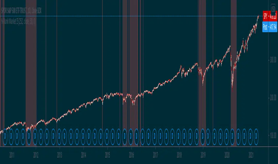
Percentile Rank Market FilterA simple script to filter bull and bear markets by using percentile rank filter. Using market regimes to filter by bull/bear/sideways markets helps to understand how your strategy will
behave in various market regimes and allows you to avoid unprofitable regimes and only trade in profitable ones.
The idea of market regime filtering is used in the most successful technical algorithmic trading strategies, as one should always design a trading strategy with a particular market in mind according to trading legend, Larry Connors
Feel free to use this script in your strategies to improve your profits and lower drawdowns.
14/28 Day SMA Divergence and RSI - No RepaintIf you are interested in purchasing my algorithmic trading bot that receives Tradingview indicator alerts via email and then executes them in Bittrex, please visit my product page here: ilikestocks.com Additionally, I would love to create video/blog guides on creating Tradingview scripts or strategies. If you are a knowledgeable in finance or other related fields and would like to be featured on my page, please contact me at tanner@ilikestocks.com.
No crossovers were used in this script, and this is likely the reason for the no repaint(Correct me if wrong).
This strategy script uses a 14-day SMA signal line, a 28-day SMA and RSI. The strategy works by determining whether the (14-day SMA is above the 28-day SMA and the RSI levels are overbought(below 30)) or RSI is very overbought(below 13 or so). Once either of these conditions have been met, a long position is opened.
The initial long position must be partially closed by the take profit first and then the final close is executed if the 14-day signal SMA is below the 28-day SMA; you may also exclusively use take profit to close positions.
The green plotted spikes are the initial long position conditions. The orange plotted spikes are take profit signals once a long position is opened. The red plotted spikes are plotted when the SMA 14-day is below the 28-day SMA.
Please do leave constructive criticism or comments below because it helps me better create scripts!

PSP Suite for Algo 1HTF -25% Target## 🔹 PSP Suite for Algo 1HTF – 25% Target
**(Nifty Options – CE / PE)**
### 📌 What this indicator is for
PSP Suite for Algo is a **trend-based directional options indicator** designed specifically for **NIFTY index options trading**.
It helps traders capture **high-probability directional moves** with **clear CE / PE signals**, controlled risk, and predefined targets.
---
## ⏱ Best Timeframe
* **Primary Timeframe:** ✅ **1 Hour (1H TF)**
* Do **not** use on lower timeframes for best accuracy
* Works best during **trending sessions**
---
## 📊 Instrument Best Suited
* **NIFTY Index**
* **NIFTY Weekly Options**
* Buy **CE** on BUY signal
* Buy **PE** on SELL signal
⚠️ Avoid Bank Nifty / Fin Nifty unless properly back-tested.
---
## 🟢 How to Trade (Simple Rules)
### ▶ BUY CE Signal
* When **BUY CE** label appears:
* Buy **ATM or slight ITM CE**
* Prefer same-week expiry
* Enter **after candle close** on 1H timeframe
### ▶ BUY PE Signal
* When **SELL PE** label appears:
* Buy **ATM or slight ITM PE**
* Prefer same-week expiry
* Enter **after candle close** on 1H timeframe
🚫 No over-trading: **Only one position per signal**
---
## 🎯 Target & Stop Loss (Strict Rule)
* **Target:** 🎯 **25% Option Premium**
* **Stop Loss:** ❌ **25% Option Premium**
* **Risk : Reward:** ⚖️ **1 : 1**
👉 When trade moves strongly in your favor, **manual trailing is recommended** (as shown on chart).
---
## 💰 Expected Returns on Nifty
* **Per Trade:**
* ~ **100 – 250 Nifty points equivalent move**
* Option premium typically gives **20–40% moves**
* **Accuracy:** High during **clear trends**
* Best results when market is **not sideways**
---
## 📅 Ideal Market Conditions
✅ Trending Market
✅ Expansion after consolidation
❌ Avoid very low-volatility / choppy sessions
---
## 🔔 Alerts
* Built-in alerts available for:
* **BUY CE**
* **BUY PE**
* Recommended to enable **Once Per Bar Close**
---
## 🧠 Important Notes
* This is **not a scalping tool**
* Designed for **positional intraday / short swing**
* Follow **discipline in SL & position sizing**
* Works best with **trend confirmation from price structure**
---
## ⚠️ Disclaimer
This indicator is for **educational and analytical purposes only**.
Options trading involves risk. Please trade responsibly.
