Kalman Filter [DCAUT]

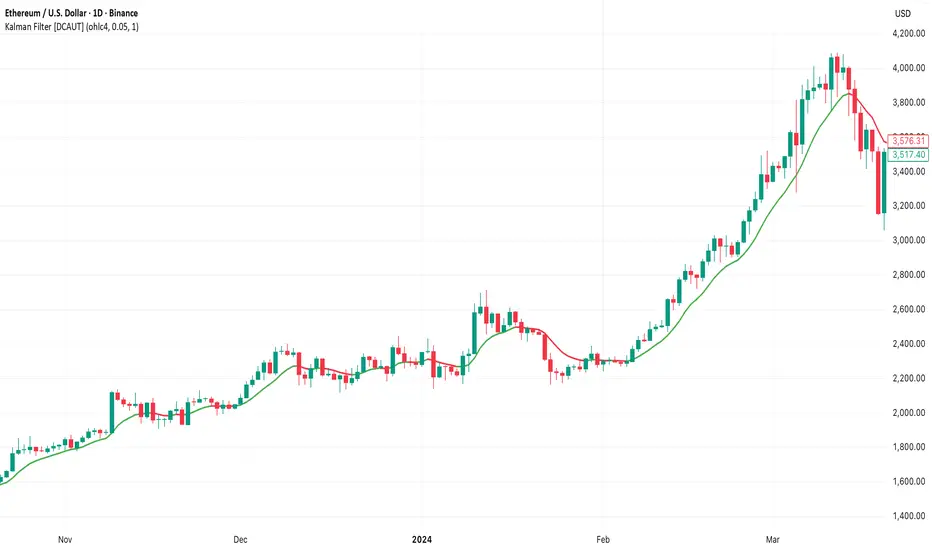
█ Kalman Filter [DCAUT]

📊 ORIGINALITY & INNOVATION

The Kalman Filter represents an important adaptation of aerospace signal processing technology to financial market analysis. Originally developed by Rudolf E. Kalman in 1960 for navigation and guidance systems, this implementation brings the algorithm's noise reduction capabilities to price trend analysis.

This implementation addresses a common challenge in technical analysis: the trade-off between smoothness and responsiveness. Traditional moving averages must choose between being smooth (with increased lag) or responsive (with increased noise). The Kalman Filter improves upon this limitation through its recursive estimation approach, which continuously balances historical trend information with current price data based on configurable noise parameters.

The key advancement lies in the algorithm's adaptive weighting mechanism. Rather than applying fixed weights to historical data like conventional moving averages, the Kalman Filter dynamically adjusts its trust between the predicted trend and observed prices. This allows it to provide smoother signals during stable periods while maintaining responsiveness during genuine trend changes, helping to reduce whipsaws in ranging markets while not missing significant price movements.

📐 MATHEMATICAL FOUNDATION

The Kalman Filter operates through a two-phase recursive process:

Prediction Phase:
The algorithm first predicts the next state based on the previous estimate:

• State Prediction: Estimates the next value based on current trend
  
• Error Covariance Prediction: Calculates uncertainty in the prediction
  

Update Phase:
Then updates the prediction based on new price observations:

• Kalman Gain Calculation: Determines the weight given to new measurements
  
• State Update: Combines prediction with observation based on calculated gain
  
• Error Covariance Update: Adjusts uncertainty estimate for next iteration
  

Core Parameters:

• Process Noise (Q): Represents uncertainty in the trend model itself. Higher values indicate the trend can change more rapidly, making the filter more responsive to price changes.
  
• Measurement Noise (R): Represents uncertainty in price observations. Higher values indicate less trust in individual price points, resulting in smoother output.
  

Kalman Gain Formula:
The Kalman Gain determines how much weight to give new observations versus predictions:
K = P(k|k-1) / (P(k|k-1) + R)

Where:

• K is the Kalman Gain (0 to 1)
  
• P(k|k-1) is the predicted error covariance
  
• R is the measurement noise parameter
  

When K approaches 1, the filter trusts new measurements more (responsive).
When K approaches 0, the filter trusts its prediction more (smooth).

This dynamic adjustment mechanism allows the filter to adapt to changing market conditions automatically, providing an advantage over fixed-weight moving averages.

📊 COMPREHENSIVE SIGNAL ANALYSIS

Visual Trend Indication:
The Kalman Filter line provides color-coded trend information:

• Green Line: Indicates the filter value is rising, suggesting upward price momentum
  
• Red Line: Indicates the filter value is falling, suggesting downward price momentum
  
• Gray Line: Indicates sideways movement with no clear directional bias
  

Crossover Signals:
Price-filter crossovers generate trading signals:

• Golden Cross: Price crosses above the Kalman Filter line, suggests potential bullish momentum development, may indicate a favorable environment for long positions, filter will naturally turn green as it adapts to price moving higher
  
• Death Cross: Price crosses below the Kalman Filter line, suggests potential bearish momentum development, may indicate consideration for position reduction or shorts, filter will naturally turn red as it adapts to price moving lower
  

Trend Confirmation:
The filter serves as a dynamic trend baseline:

• Price Consistently Above Filter: Confirms established uptrend
  
• Price Consistently Below Filter: Confirms established downtrend
  
• Frequent Crossovers: Suggests ranging or choppy market conditions
  

Signal Reliability Factors:
Signal quality varies based on market conditions:

• Higher reliability in trending markets with sustained directional moves
  
• Lower reliability in choppy, range-bound conditions with frequent reversals
  
• Parameter adjustment can help adapt to different market volatility levels
  

🎯 STRATEGIC APPLICATIONS

Trend Following Strategy:
Use the Kalman Filter as a dynamic trend baseline:

1. Enter long positions when price crosses above the filter
   
2. Enter short positions when price crosses below the filter
   
3. Exit when price crosses back through the filter in the opposite direction
   
4. Monitor filter slope (color) for trend strength confirmation
   

Dynamic Support/Resistance:
The filter can act as a moving support or resistance level:

• In uptrends: Filter often provides dynamic support for pullbacks
  
• In downtrends: Filter often provides dynamic resistance for bounces
  
• Price rejections from the filter can offer entry opportunities in trend direction
  
• Filter breaches may signal potential trend reversals
  

Multi-Timeframe Analysis:
Combine Kalman Filters across different timeframes:

• Higher timeframe filter identifies primary trend direction
  
• Lower timeframe filter provides precise entry and exit timing
  
• Trade only in direction of higher timeframe trend for better probability
  
• Use lower timeframe crossovers for position entry/exit within major trend
  

Volatility-Adjusted Configuration:
Adapt parameters to match market conditions:

• Low Volatility Markets (Forex majors, stable stocks): Use lower process noise for stability, use lower measurement noise for sensitivity
  
• Medium Volatility Markets (Most equities): Process noise default (0.05) provides balanced performance, measurement noise default (1.0) for general-purpose filtering
  
• High Volatility Markets (Cryptocurrencies, volatile stocks): Use higher process noise for responsiveness, use higher measurement noise for noise reduction
  

Risk Management Integration:

• Use filter as a trailing stop-loss level in trending markets
  
• Tighten stops when price moves significantly away from filter (overextension)
  
• Wider stops in early trend formation when filter is just establishing direction
  
• Consider position sizing based on distance between price and filter
  

📋 DETAILED PARAMETER CONFIGURATION

Source Selection:
Determines which price data feeds the algorithm:

• OHLC4 (default): Uses average of open, high, low, close for balanced representation
  
• Close: Focuses purely on closing prices for end-of-period analysis
  
• HL2: Uses midpoint of high and low for range-based analysis
  
• HLC3: Typical price, gives more weight to closing price
  
• HLCC4: Weighted close price, emphasizes closing values
  

Process Noise (Q) - Adaptation Speed Control:
This parameter controls how quickly the filter adapts to changes:

Technical Meaning:

• Represents uncertainty in the underlying trend model
  
• Higher values allow the estimated trend to change more rapidly
  
• Lower values assume the trend is more stable and slow-changing
  

Practical Impact:

• Lower Values: Produces very smooth output with minimal noise, slower to respond to genuine trend changes, best for long-term trend identification, reduces false signals in choppy markets
  
• Medium Values: Balanced responsiveness and smoothness, suitable for swing trading applications, default (0.05) works well for most markets
  
• Higher Values: More responsive to price changes, may produce more false signals in ranging markets, better for short-term trading and day trading, captures trend changes earlier, adjust freely based on market characteristics
  

Measurement Noise (R) - Smoothing Control:
This parameter controls how much the filter trusts individual price observations:

Technical Meaning:

• Represents uncertainty in price measurements
  
• Higher values indicate less trust in individual price points
  
• Lower values make each price observation more influential
  

Practical Impact:

• Lower Values: More reactive to each price change, less smoothing with more noise in output, may produce choppy signals
  
• Medium Values: Balanced smoothing and responsiveness, default (1.0) provides general-purpose filtering
  
• Higher Values: Heavy smoothing for very noisy markets, reduces whipsaws significantly but increases lag in trend change detection, best for cryptocurrency and highly volatile assets, can use larger values for extreme smoothing
  

Parameter Interaction:
The ratio between Process Noise and Measurement Noise determines overall behavior:

• High Q / Low R: Very responsive, minimal smoothing
  
• Low Q / High R: Very smooth, maximum lag reduction
  
• Balanced Q and R: Middle ground for most applications
  

Optimization Guidelines:

1. Start with default values (Q=0.05, R=1.0)
   
2. If too many false signals: Increase R or decrease Q
   
3. If missing trend changes: Decrease R or increase Q
   
4. Test across different market conditions before live use
   
5. Consider different settings for different timeframes
   

📈 PERFORMANCE ANALYSIS & COMPETITIVE ADVANTAGES

Comparison with Traditional Moving Averages:

Versus Simple Moving Average (SMA):

• The Kalman Filter typically responds faster to genuine trend changes
  
• Produces smoother output than SMA of comparable length
  
• Better noise reduction in ranging markets
  
• More configurable for different market conditions
  

Versus Exponential Moving Average (EMA):

• Similar responsiveness but with better noise filtering
  
• Less prone to whipsaws in choppy conditions
  
• More adaptable through dual parameter control (Q and R)
  
• Can be tuned to match or exceed EMA responsiveness while maintaining smoothness
  

Versus Hull Moving Average (HMA):

• Different noise reduction approach (recursive estimation vs. weighted calculation)
  
• Kalman Filter offers more intuitive parameter adjustment
  
• Both reduce lag effectively, but through different mechanisms
  
• Kalman Filter may handle sudden volatility changes more gracefully
  

Response Characteristics:

• Lag Time: Moderate and configurable through parameter adjustment
  
• Noise Reduction: Good to excellent, particularly in volatile conditions
  
• Trend Detection: Effective across multiple timeframes
  
• False Signal Rate: Typically lower than simple moving averages in ranging markets
  
• Computational Efficiency: Efficient recursive calculation suitable for real-time use
  

Optimal Use Cases:

• Markets with mixed trending and ranging periods
  
• Assets with moderate to high volatility requiring noise filtering
  
• Multi-timeframe analysis requiring consistent methodology
  
• Systematic trading strategies needing reliable trend identification
  
• Situations requiring balance between responsiveness and smoothness
  

Known Limitations:

• Parameters require adjustment for different market volatility levels
  
• May still produce false signals during extreme choppy conditions
  
• No single parameter set works optimally for all market conditions
  
• Requires complementary indicators for comprehensive analysis
  
• Historical performance characteristics may not persist in changing market conditions
  

USAGE NOTES

This indicator is designed for technical analysis and educational purposes. The Kalman Filter's effectiveness varies with market conditions, tending to perform better in markets with clear trending phases interrupted by consolidation. Like all technical indicators, it has limitations and should not be used as the sole basis for trading decisions, but rather as part of a comprehensive trading approach.

Algorithm performance varies with market conditions, and past characteristics do not guarantee future results. Always test thoroughly with different parameter settings across various market conditions before using in live trading. No technical indicator can predict future price movements with certainty, and all trading involves risk of loss.