Mutanabby_AI | ONEUSDT_MR1
ONEUSDT Mean-Reversion Strategy | 74.68% Win Rate | 417% Net Profit
This is a long-only mean-reversion strategy designed specifically for ONEUSDT on the 1-hour timeframe. The core logic identifies oversold conditions following sharp declines and enters positions when selling pressure exhausts, capturing the subsequent recovery bounce.
Backtested Period: June 2019 – December 2025 (~6 years)
Performance Summary
| Metric | Value |
|--------|-------|
| Net Profit | +417.68% |
| Win Rate | 74.68% |
| Profit Factor | 4.019 |
| Total Trades | 237 |
| Sharpe Ratio | 0.364 |
| Sortino Ratio | 1.917 |
| Max Drawdown | 51.08% |
| Avg Win | +3.14% |
| Avg Loss | -2.30% |
| Buy & Hold Return | -80.44% |
Strategy Logic :
Entry Conditions (Long Only):
The strategy seeks confluence of three conditions that identify exhausted selling:
1. Prior Move Filter:*The price change from 5 bars ago to 3 bars ago must be ≥ -7% (ensures we're not entering during freefall)
2. Current Move Filter: The price change over the last 2 bars must be ≤ 0% (confirms momentum is stalling or reversing)
3. Three-Bar Decline: The price change from 5 bars ago to 3 bars ago must be ≤ -5% (confirms a significant recent drop occurred)
When all three conditions align, the strategy identifies a potential reversal point where sellers are exhausted.
Exit Conditions:
- Primary Exit: Close above the previous bar's high while the open of the previous bar is at or below the close from 9 bars ago (profit-taking on strength)
- Trailing Stop: 11x ATR trailing stop that locks in profits as price rises
Risk Management
- Position Sizing:Fixed position based on account equity divided by entry price
- Trailing Stop:11× ATR (14-period) provides wide enough room for crypto volatility while protecting gains
- Pyramiding:Up to 4 orders allowed (can scale into winning positions)
- **Commission:** 0.1% per trade (realistic exchange fees included)
Important Disclaimers
⚠️ This is NOT financial advice.
- Past performance does not guarantee future results
- Backtest results may contain look-ahead bias or curve-fitting
- Real trading involves slippage, liquidity issues, and execution delays
- This strategy is optimized for ONEUSDT specifically — results may differ on other pairs
- Always test before risking real capital
Recommended Usage
- Timeframe:*1H (as designed)
- Pair: ONEUSDT (Binance)
- Account Size: Ensure sufficient capital to survive max drawdown
Source Code
Feedback Welcome
I'm sharing this strategy freely for educational purposes. Please:
- Drop a comment with your backtesting results any you analysis
- Share any modifications that improve performance
- Let me know if you spot any issues in the logic
Happy trading
As a quant trader, do you think this strategy will survive in live trading?
Yes or No? And why?
I want to hear from you guys
BTCUSD

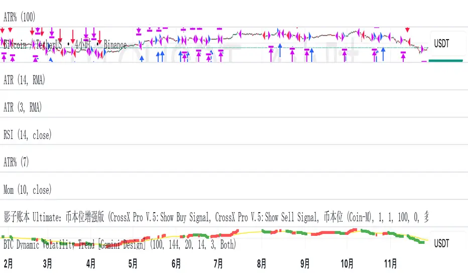
BTC Dynamic Volatility Trend Backtested from 2017 to present, this strategy has delivered a staggering 7100%+ cumulative return. It doesn't just track the market; it dominates it. By capturing major trends and strictly limiting drawdowns, it has significantly outperformed the standard 'Buy & Hold' BTC strategy, proving its ability to generate massive alpha across multiple bull and bear cycles.
自 2017 年至今,本策略实现了惊人的 7100%+ 累计收益率。它不仅仅是跟随市场,更是超越了市场。通过精准捕捉主升浪并严格控制回撤,该策略在穿越多轮牛熊周期后,大幅度跑赢了比特币‘买入持有’(Buy & Hold)的基准收益,展现了极致的阿尔法(Alpha)捕捉能力。"
Introduction :Simplicity is the ultimate sophistication. This strategy is designed specifically for Bitcoin (BTC), capturing its unique characteristics: high volatility, frequent fakeouts, and massive trend persistence. It abandons complex indicators in favor of a robust logic: "Follow the Trend, Filter the Noise, Let Profits Run."
Core Logic
Trend Filter (Fibonacci EMA 144): We use the 144-period Exponential Moving Average as the baseline. Longs are only taken above this line, and shorts only below. This keeps you on the right side of the major trend.
Volatility Breakout (Donchian Channel 20): Entries are triggered only when price breaks the 20-day high (for longs) or low (for shorts). This confirms momentum and avoids trading in chop.
Dynamic Risk Management (ATR Chandelier Exit):
Instead of fixed % stops, we use Average True Range (ATR) to calculate stop losses.
The Ratchet Mechanism: The stop loss moves up with the price but never moves down (for longs). This locks in profits automatically as the trend develops and exits immediately when volatility turns against you.
Why Use This Strategy?
Zero Repainting: All signals are confirmed.
No Curve Fitting: Uses classic parameters (144, 20) that have worked for decades.
Mental Peace: The strategy handles the exit. You don't need to guess where to sell. It holds through minor corrections and exits only when the trend truly reverses.
Settings
Leverage %: Adjust your position size based on equity (default 100% = 1x).
Timeframe: Recommended for 4H charts.
中文版 (Chinese Version)
简介 :大道至简。本策略专为 比特币 (BTC) 设计,针对其高波动、假突破多但趋势爆发力强的特点,摒弃了复杂的过度拟合指标,回归交易本质:“顺大势,滤噪音,截断亏损,让利润奔跑”。
核心逻辑
趋势过滤器 (斐波那契 EMA 144): 使用 144 周期指数移动平均线作为多空分水岭。价格在均线之上只做多,之下只做空。这能有效过滤掉大部分震荡市的噪音。
波动率突破 (唐奇安通道 20): 只有当价格突破过去 20 根 K 线的最高价(做多)或最低价(做空)时才进场。这确保了我们只在趋势确立的瞬间入场。
动态风控 (ATR 吊灯止损):
拒绝固定点数止损,使用 ATR(平均真实波幅)根据市场热度动态计算安全距离。
棘轮机制: 止损线会跟随价格上涨而上移,但绝不会下移(做多时)。这实现了自动化的“利润锁定”,既能扛住正常的波动回调,又能在大势反转时果断离场。
策略优势
绝不重绘: 所有信号均为收盘确认或实时触价。
拒绝拟合: 使用经过数十年市场验证的经典参数组合。
心态管理: 策略全自动管理出场。你不需要纠结何时止盈,它会帮你吃到完整的鱼身,直到趋势结束。
使用建议
资金管理: 可通过参数调整仓位占比(默认 100% = 1倍杠杆)。
推荐周期: 建议在4小时 图表上运行效果最佳。
Crypto Scalping Strategy by SAIFOverview
An optimized scalping strategy designed for cryptocurrency markets, focusing on breakout opportunities with strict risk controls and optional safe compounding features. This strategy combines price action, volume analysis, and multi-timeframe trend confirmation.
Key Features
Breakout Detection System
Identifies significant price breakouts using dynamic channel analysis
Confirms breakouts with volume surge validation
Filters trades based on multi-timeframe trend alignment
Multi-Timeframe Trend Confirmation
Analyzes 1-hour and 4-hour timeframes for trend direction
Only takes trades aligned with higher timeframe trends
Uses long-term moving averages for trend validation
Advanced Risk Management
Conservative default risk: 1% per trade
ATR-based stop-loss placement (2x ATR)
Trailing stop mechanism to protect profits
Minimum profit target before trailing activates
Built-in position sizing based on account equity
Safe Capital Management Options
Fixed Capital Mode: Trade with consistent position sizes
Safe Compounding Mode: Gradually scales position size based on realized profits only
Drawdown Protection: 80% equity floor prevents excessive capital erosion
Leverage Control: 10x leverage factored into position calculations
Technical Filters
Momentum confirmation via oscillator conditions
Directional movement analysis
Volume threshold requirements
Trend strength validation
Position Sizing
The strategy automatically calculates position sizes based on:
Your specified risk percentage
Current ATR volatility
Available leverage
Account equity (with optional compounding)
Trade Management
Entry: Executes on confirmed breakouts with volume and trend alignment
Stop Loss: Placed at 2x ATR from entry
Take Profit: Uses trailing stops that activate after minimum profit threshold
Exit: Automatically managed through strategy exits
Customization Options
Adjustable channel length for breakout detection
Configurable volume multiplier for surge detection
Customizable oscillator thresholds
Flexible ATR period for volatility measurement
Optional compounding vs. fixed capital modes
Adjustable trailing stop parameters
Visual Features
Channel boundaries plotted on chart
Entry signals marked with arrows
Background coloring indicates trend direction
Real-time info table shows:
Current risk level
Compounding status
Capital values
Drawdown protection status
Alert Capabilities
Built-in alert conditions for:
Buy signals (breakout opportunities)
Sell signals (breakdown opportunities)
Important Disclaimers
⚠️ Educational Purpose Only: This strategy is provided for educational and research purposes. It is not investment advice.
⚠️ High-Risk Trading: Scalping and leverage trading carry substantial risk of loss. Cryptocurrency markets are highly volatile.
⚠️ Not Financial Advice: This tool does not constitute financial, investment, or trading advice. Always conduct your own research and consult qualified professionals.
⚠️ Leverage Warning: This strategy uses 10x leverage, which can amplify both gains and losses significantly.
⚠️ Backtesting Limitations: Past performance does not guarantee future results. Real trading involves slippage, execution delays, and emotional factors not present in backtesting.
⚠️ Capital at Risk: Only trade with capital you can afford to lose completely. Never trade with borrowed money or funds needed for living expenses.
Commission & Fees
Commission: 0.13% per trade
Initial capital: $100 (default)
Commission costs are factored into backtest results
Best Practices
Start Small: Begin with minimum capital and conservative risk settings
Test Thoroughly: Backtest across different market conditions and timeframes
Monitor Performance: Track win rate, profit factor, and maximum drawdown
Adjust Parameters: Optimize settings for your specific trading pairs
Use Alerts: Set up notifications to avoid missing opportunities
Manage Emotions: Follow the strategy rules consistently without override
Recommended Markets
High liquidity cryptocurrency pairs (BTC, ETH major pairs)
Assets with clear trending behavior
Markets with sufficient volume for scalping
Timeframes: 1H to 4H charts recommended
Risk Reminder
Scalping requires:
Quick decision-making
Tight risk management
Consistent discipline
Understanding of market microstructure
Proper capitalization
Always practice proper risk management. The strategy includes safety features, but no system can eliminate trading risk entirely. Trade responsibly.


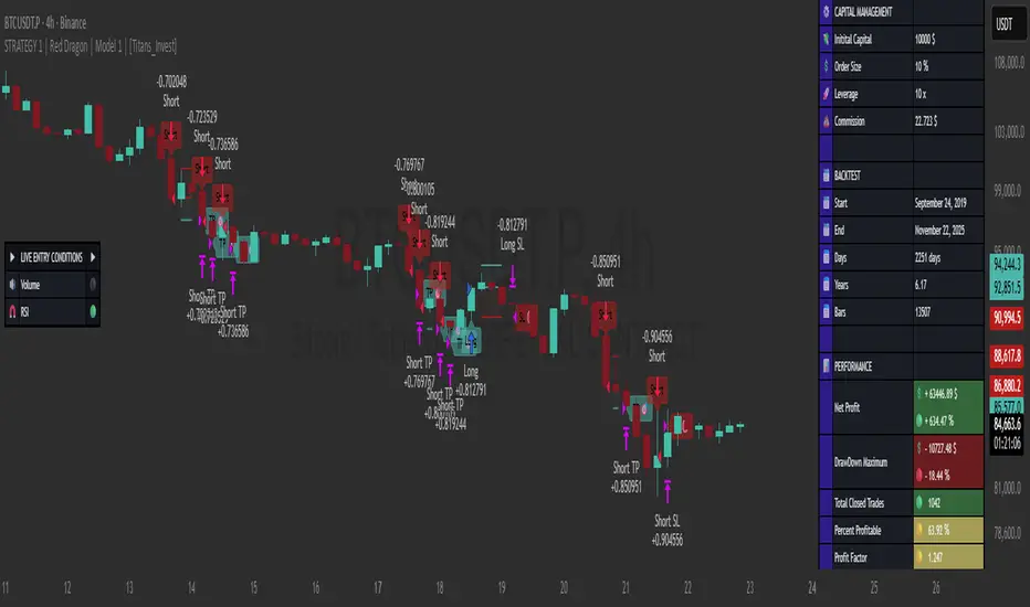
STRATEGY 1 │ Red Dragon │ Model 1 │ [Titans_Invest]The Red Dragon Model 1 is a fully automated trading strategy designed to operate BTC/USDT.P on the 4-hour chart with precision, stability, and consistency. It was built to deliver reliable behavior even during strong market movements, maintaining operational discipline and avoiding abrupt variations that could interfere with the trader’s decision-making.
Its core is based on a professionally engineered logical structure that combines trend filters, confirmation criteria, and balanced risk management. Every component was designed to work in an integrated way, eliminating noise, avoiding unnecessary trades, and protecting capital in critical moments. There are no secret mechanisms or hidden logic: everything is built to be objective, clean, and efficient.
Even though it is based on professional quantitative engineering, Red Dragon Model 1 remains extremely simple to operate. All logic is clearly displayed and fully accessible within TradingView itself, making it easy to understand for both beginners and experienced traders. The structure is organized so that any user can quickly view entry conditions, exit criteria, additional filters, adjustable parameters, and the full mechanics behind the strategy’s behavior.
In addition, the architecture was built to minimize unnecessary complexity. Parameters are straightforward, intuitive, and operate in a balanced way without requiring deep adjustments or advanced knowledge. Traders have full freedom to analyze the strategy, understand the logic, and make personal adaptations if desired—always with total transparency inside TradingView.
The strategy was also designed to deliver consistent operational behavior over the long term. Its confirmation criteria reduce impulsive trades; its filters isolate noise; and its overall logic prioritizes high-quality entries in structured market movements. The goal is to provide a stable, clear, and repeatable flow—essential characteristics for any medium-term quantitative approach.
Combining clarity, professional structure, and ease of use, Red Dragon Model 1 offers a solid foundation both for users who want a ready-to-use automated strategy and for those looking to study quantitative models in greater depth.
This entire project was built with extreme dedication, backed by more than 14,000 hours of hands-on experience in Pine Script, continuously refining patterns, techniques, and structures until reaching its current level of maturity. Every line of code reflects this long process of improvement, resulting in a strategy that unites professional engineering, transparency, accessibility, and reliable execution.
🔶 MAIN FEATURES
• Fully automated and robust: Operates without manual intervention, ideal for traders seeking consistency and stability. It delivers reliable performance even in volatile markets thanks to the solid quantitative engineering behind the system.
• Multiple layers of confirmation: Combines 10 key technical indicators with 15 adaptive filters to avoid false signals. It only triggers entries when all trend, market strength, and contextual criteria align.
• Configurable and adaptable filters: Each of the 15 filters can be enabled, disabled, or adjusted by the user, allowing the creation of personalized statistical models for different assets and timeframes. This flexibility gives full freedom to optimize the strategy according to individual preferences.
• Clear and accessible logic: All entry and exit conditions are explicitly shown within the TradingView parameters. The strategy has no hidden components—any user can quickly analyze and understand each part of the system.
• Integrated exclusive tools: Includes complete backtest tables (desktop and mobile versions) with annualized statistics, along with real-time entry conditions displayed directly on the chart. These tools help monitor the strategy across devices and track performance and risk metrics.
• No repaint: All signals are static and do not change after being plotted. This ensures the trader can trust every entry shown without worrying about indicators rewriting past values.
🔷 ENTRY CONDITIONS & RISK MANAGEMENT
Red Dragon Model 1 triggers buy (long) or sell (short) signals only when all configured conditions are satisfied. For example:
• Volume:
• The system only trades when current volume exceeds the volume moving average multiplied by a user-defined factor, indicating meaningful market participation.
• RSI:
• Confirms bullish bias when RSI crosses above its moving average, and bearish bias when crossing below.
• ADX:
• Enters long when +DI is above –DI with ADX above a defined threshold, indicating directional strength to the upside (and the opposite conditions for shorts).
• Other indicators (MACD, SAR, Ichimoku, Support/Resistance, etc.)
Each one must confirm the expected direction before a final signal is allowed.
When all bullish criteria are met simultaneously, the system enters Long; when all criteria indicate a bearish environment, the system enters Short.
In addition, the strategy uses fixed Take Profit and Stop Loss targets for risk control:
Currently: TP around 1.5% and SL around 2.0% per trade, ensuring consistent and transparent risk management on every position.
⚙️ INDICATORS
__________________________________________________________
1) 🔊 Volume: Avoids trading on flat charts.
2) 🍟 MACD: Tracks momentum through moving averages.
3) 🧲 RSI: Indicates overbought or oversold conditions.
4) 🅰️ ADX: Measures trend strength and potential entry points.
5) 🥊 SAR: Identifies changes in price direction.
6) ☁️ Cloud: Accurately detects changes in market trends.
7) 🌡️ R/F: Improves trend visualization and helps avoid pitfalls.
8) 📐 S/R: Fixed support and resistance levels.
9)╭╯MA: Moving Averages.
10) 🔮 LR: Forecasting using Linear Regression.
__________________________________________________________
🟢 ENTRY CONDITIONS 🔴
__________________________________________________________
IF all conditions are 🟢 = 📈 Long
IF all conditions are 🔴 = 📉 Short
__________________________________________________________
🚨 CURRENT TRIGGER SIGNAL 🚨
__________________________________________________________
🔊 Volume
🟢 LONG = (volume) > (MA_volume) * (Volume Mult)
🔴 SHORT = (volume) > (MA_volume) * (Volume Mult)
🧲 RSI
🟢 LONG = (RSI) > (RSI_MA)
🔴 SHORT = (RSI) < (RSI_MA)
🟢 ALL ENTRY CONDITIONS AVAILABLE 🔴
__________________________________________________________
🔊 Volume
🟢 LONG = (volume) > (MA_volume) * (Volume Mult)
🔴 SHORT = (volume) > (MA_volume) * (Volume Mult)
🔊 Volume
🟢 LONG = (volume) > (MA_volume) * (Volume Mult) and (close) > (open)
🔴 SHORT = (volume) > (MA_volume) * (Volume Mult) and (close) < (open)
🍟 MACD
🟢 LONG = (MACD) > (Signal Smoothing)
🔴 SHORT = (MACD) < (Signal Smoothing)
🧲 RSI
🟢 LONG = (RSI) < (Upper)
🔴 SHORT = (RSI) > (Lower)
🧲 RSI
🟢 LONG = (RSI) > (RSI_MA)
🔴 SHORT = (RSI) < (RSI_MA)
🅰️ ADX
🟢 LONG = (+DI) > (-DI) and (ADX) > (Treshold)
🔴 SHORT = (+DI) < (-DI) and (ADX) > (Treshold)
🥊 SAR
🟢 LONG = (close) > (SAR)
🔴 SHORT = (close) < (SAR)
☁️ Cloud
🟢 LONG = (Cloud A) > (Cloud B)
🔴 SHORT = (Cloud A) < (Cloud B)
☁️ Cloud
🟢 LONG = (Kama) > (Kama )
🔴 SHORT = (Kama) < (Kama )
🌡️ R/F
🟢 LONG = (high) > (UP Range) and (upward) > (0)
🔴 SHORT = (low) < (DOWN Range) and (downward) > (0)
🌡️ R/F
🟢 LONG = (high) > (UP Range)
🔴 SHORT = (low) < (DOWN Range)
📐 S/R
🟢 LONG = (close) > (Resistance)
🔴 SHORT = (close) < (Support)
╭╯MA2️⃣
🟢 LONG = (Cyan Bar MA2️⃣)
🔴 SHORT = (Red Bar MA2️⃣)
╭╯MA2️⃣
🟢 LONG = (close) > (MA2️⃣)
🔴 SHORT = (close) < (MA2️⃣)
╭╯MA2️⃣
🟢 LONG = (Positive MA2️⃣)
🔴 SHORT = (Negative MA2️⃣)
__________________________________________________________
🎯 TP / SL 🛑
__________________________________________________________
🎯 TP: 1.5 %
🛑 SL: 2.0 %
__________________________________________________________
🪄 UNIQUE FEATURES OF THIS STRATEGY
____________________________________
1) 𝄜 Table Backtest for Mobile.
2) 𝄜 Table Backtest for Computer.
3) 𝄜 Table Backtest for Computer & Annual Performance.
4) 𝄜 Live Entry Conditions.
1) 𝄜 Table Backtest for Mobile.
2) 𝄜 Table Backtest for Computer.
3) 𝄜 Table Backtest for Computer & Annual Performance.
4) 𝄜 Live Entry Conditions.
_____________________________
𝄜 BACKTEST / PERFORMANCE 𝄜
_____________________________
• Net Profit: +634.47%, Maximum Drawdown: -18.44%.
🪙 PAIR / TIMEFRAME ⏳
🪙 PAIR: BINANCE:BTCUSDT.P
⏳ TIME: 4 hours (240m)
✅ ON ☑️ OFF
✅ LONG
✅ SHORT
🎯 TP / SL 🛑
🎯 TP: 1.5 (%)
🛑 SL: 2.0 (%)
⚙️ CAPITAL MANAGEMENT
💸 Initial Capital: 10000 $ (TradingView)
💲 Order Size: 10 % (Of Equity)
🚀 Leverage: 10 x (Exchange)
💩 Commission: 0.03 % (Exchange)
📆 BACKTEST
🗓️ Start: Setember 24, 2019
🗓️ End: November 21, 2025
🗓️ Days: 2250
🗓️ Yers: 6.17
🗓️ Bars: 13502
📊 PERFORMANCE
💲 Net Profit: + 63446.89 $
🟢 Net Profit: + 634.47 %
💲 DrawDown Maximum: - 10727.48 $
🔴 DrawDown Maximum: - 18.44 %
🟢 Total Closed Trades: 1042
🟡 Percent Profitable: 63.92 %
🟡 Profit Factor: 1.247
💲 Avg Trade: + 60.89 $
⏱️ Avg # Bars in Trades
🕯️ Avg # Bars: 4
⏳ Avg # Hrs: 15
✔️ Trades Winning: 666
❌ Trades Losing: 376
✔️ Maximum Consecutive Wins: 11
❌ Maximum Consecutive Losses: 7
📺 Live Performance : br.tradingview.com
• Use this strategy on the recommended pair and timeframe above to replicate the tested results.
• Feel free to experiment and explore other settings, assets, and timeframes.
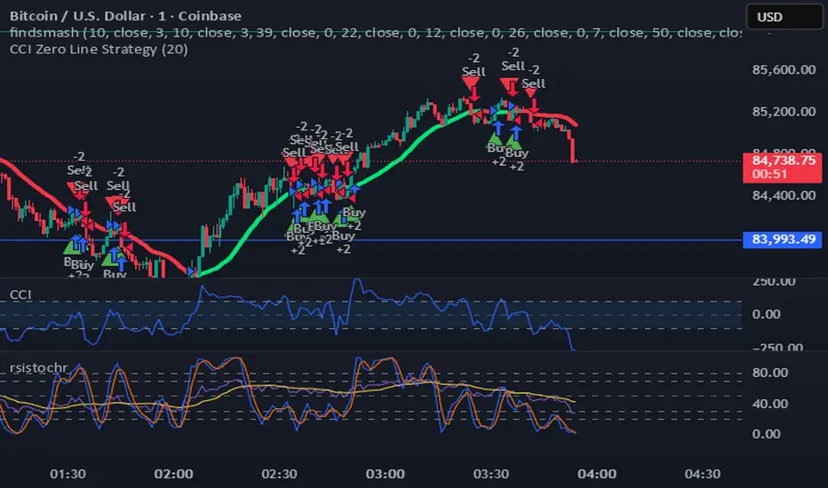
CCI Zero Line StrategyCCI Zero Line Strategy i have created this using cci just check in different time frame you and check the results

WMAX-D-TPS1 (USD setup)Here I show you a strategy that I have been developing for years based on breakouts of maximum and minimum price levels.This work good in 1d

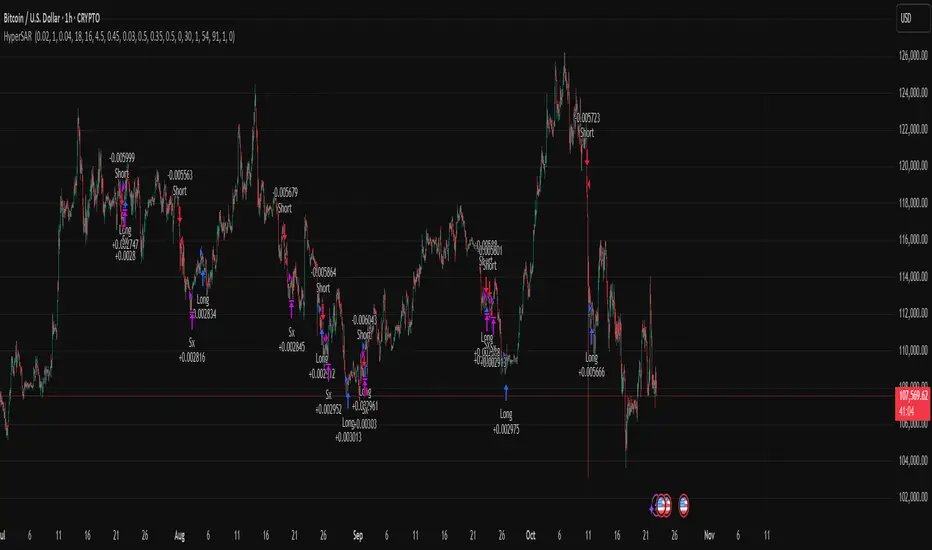
Hyper SAR Reactor Trend StrategyHyperSAR Reactor Adaptive PSAR Strategy
Summary
Adaptive Parabolic SAR strategy for liquid stocks, ETFs, futures, and crypto across intraday to daily timeframes. It acts only when an adaptive trail flips and confirmation gates agree. Originality comes from a logistic boost of the SAR acceleration using drift versus ATR, plus ATR hysteresis, inertia on the trail, and a bear-only gate for shorts. Add to a clean chart and run on bar close for conservative alerts.
Scope and intent
• Markets: large cap equities and ETFs, index futures, major FX, liquid crypto
• Timeframes: one minute to daily
• Default demo: BTC on 60 minute
• Purpose: faster yet calmer PSAR that resists chop and improves short discipline
• Limits: this is a strategy that places simulated orders on standard candles
Originality and usefulness
• Novel fusion: PSAR AF is boosted by a logistic function of normalized drift, trail is monotone with inertia, entries use ATR buffers and optional cooldown, shorts are allowed only in a bear bias
• Addresses false flips in low volatility and weak downtrends
• All controls are exposed in Inputs for testability
• Yardstick: ATR normalizes drift so settings port across symbols
• Open source. No links. No solicitation
Method overview
Components
• Adaptive AF: base step plus boost factor times logistic strength
• Trail inertia: one sided blend that keeps the SAR monotone
• Flip hysteresis: price must clear SAR by a buffer times ATR
• Volatility gate: ATR over its mean must exceed a ratio
• Bear bias for shorts: price below EMA of length 91 with negative slope window 54
• Cooldown bars optional after any entry
• Visual SAR smoothing is cosmetic and does not drive orders
Fusion rule
Entry requires the internal flip plus all enabled gates. No weighted scores.
Signal rule
• Long when trend flips up and close is above SAR plus buffer times ATR and gates pass
• Short when trend flips down and close is below SAR minus buffer times ATR and gates pass
• Exit uses SAR as stop and optional ATR take profit per side
Inputs with guidance
Reactor Engine
• Start AF 0.02. Lower slows new trends. Higher reacts quicker
• Max AF 1. Typical 0.2 to 1. Caps acceleration
• Base step 0.04. Typical 0.01 to 0.08. Raises speed in trends
• Strength window 18. Typical 10 to 40. Drift estimation window
• ATR length 16. Typical 10 to 30. Volatility unit
• Strength gain 4.5. Typical 2 to 6. Steepness of logistic
• Strength center 0.45. Typical 0.3 to 0.8. Midpoint of logistic
• Boost factor 0.03. Typical 0.01 to 0.08. Adds to step when strength rises
• AF smoothing 0.50. Typical 0.2 to 0.7. Adds inertia to AF growth
• Trail smoothing 0.35. Typical 0.15 to 0.45. Adds inertia to the trail
• Allow Long, Allow Short toggles
Trade Filters
• Flip confirm buffer ATR 0.50. Typical 0.2 to 0.8. Raise to cut flips
• Cooldown bars after entry 0. Typical 0 to 8. Blocks re entry for N bars
• Vol gate length 30 and Vol gate ratio 1. Raise ratio to trade only in active regimes
• Gate shorts by bear regime ON. Bear bias window 54 and Bias MA length 91 tune strictness
Risk
• TP long ATR 1.0. Set to zero to disable
• TP short ATR 0.0. Set to 0.8 to 1.2 for quicker shorts
Usage recipes
Intraday trend focus
Confirm buffer 0.35 to 0.5. Cooldown 2 to 4. Vol gate ratio 1.1. Shorts gated by bear regime.
Intraday mean reversion focus
Confirm buffer 0.6 to 0.8. Cooldown 4 to 6. Lower boost factor. Leave shorts gated.
Swing continuation
Strength window 24 to 34. ATR length 20 to 30. Confirm buffer 0.4 to 0.6. Use daily or four hour charts.
Properties visible in this publication
Initial capital 10000. Base currency USD. Order size Percent of equity 3. Pyramiding 0. Commission 0.05 percent. Slippage 5 ticks. Process orders on close OFF. Bar magnifier OFF. Recalculate after order filled OFF. Calc on every tick OFF. No security calls.
Realism and responsible publication
No performance claims. Past results never guarantee future outcomes. Shapes can move while a bar forms and settle on close. Strategies execute only on standard candles.
Honest limitations and failure modes
High impact events and thin books can void assumptions. Gap heavy symbols may prefer longer ATR. Very quiet regimes can reduce contrast and invite false flips.
Open source reuse and credits
Public domain building blocks used: PSAR concept and ATR. Implementation and fusion are original. No borrowed code from other authors.
Strategy notice
Orders are simulated on standard candles. No lookahead.
Entries and exits
Long: flip up plus ATR buffer and all gates true
Short: flip down plus ATR buffer and gates true with bear bias when enabled
Exit: SAR stop per side, optional ATR take profit, optional cooldown after entry
Tie handling: stop first if both stop and target could fill in one bar
Quantum Flux Universal Strategy Summary in one paragraph
Quantum Flux Universal is a regime switching strategy for stocks, ETFs, index futures, major FX pairs, and liquid crypto on intraday and swing timeframes. It helps you act only when the normalized core signal and its guide agree on direction. It is original because the engine fuses three adaptive drivers into the smoothing gains itself. Directional intensity is measured with binary entropy, path efficiency shapes trend quality, and a volatility squash preserves contrast. Add it to a clean chart, watch the polarity lane and background, and trade from positive or negative alignment. For conservative workflows use on bar close in the alert settings when you add alerts in a later version.
Scope and intent
• Markets. Large cap equities and ETFs. Index futures. Major FX pairs. Liquid crypto
• Timeframes. One minute to daily
• Default demo used in the publication. QQQ on one hour
• Purpose. Provide a robust and portable way to detect when momentum and confirmation align, while dampening chop and preserving turns
• Limits. This is a strategy. Orders are simulated on standard candles only
Originality and usefulness
• Unique concept or fusion. The novelty sits in the gain map. Instead of gating separate indicators, the model mixes three drivers into the adaptive gains that power two one pole filters. Directional entropy measures how one sided recent movement has been. Kaufman style path efficiency scores how direct the path has been. A volatility squash stabilizes step size. The drivers are blended into the gains with visible inputs for strength, windows, and clamps.
• What failure mode it addresses. False starts in chop and whipsaw after fast spikes. Efficiency and the squash reduce over reaction in noise.
• Testability. Every component has an input. You can lengthen or shorten each window and change the normalization mode. The polarity plot and background provide a direct readout of state.
• Portable yardstick. The core is normalized with three options. Z score, percent rank mapped to a symmetric range, and MAD based Z score. Clamp bounds define the effective unit so context transfers across symbols.
Method overview in plain language
The strategy computes two smoothed tracks from the chart price source. The fast track and the slow track use gains that are not fixed. Each gain is modulated by three drivers. A driver for directional intensity, a driver for path efficiency, and a driver for volatility. The difference between the fast and the slow tracks forms the raw flux. A small phase assist reduces lag by subtracting a portion of the delayed value. The flux is then normalized. A guide line is an EMA of a small lead on the flux. When the flux and its guide are both above zero, the polarity is positive. When both are below zero, the polarity is negative. Polarity changes create the trade direction.
Base measures
• Return basis. The step is the change in the chosen price source. Its absolute value feeds the volatility estimate. Mean absolute step over the window gives a stable scale.
• Efficiency basis. The ratio of net move to the sum of absolute step over the window gives a value between zero and one. High values mean trend quality. Low values mean chop.
• Intensity basis. The fraction of up moves over the window plugs into binary entropy. Intensity is one minus entropy, which maps to zero in uncertainty and one in very one sided moves.
Components
• Directional Intensity. Measures how one sided recent bars have been. Smoothed with RMA. More intensity increases the gain and makes the fast and slow tracks react sooner.
• Path Efficiency. Measures the straightness of the price path. A gamma input shapes the curve so you can make trend quality count more or less. Higher efficiency lifts the gain in clean trends.
• Volatility Squash. Normalizes the absolute step with Z score then pushes it through an arctangent squash. This caps the effect of spikes so they do not dominate the response.
• Normalizer. Three modes. Z score for familiar units, percent rank for a robust monotone map to a symmetric range, and MAD based Z for outlier resistance.
• Guide Line. EMA of the flux with a small lead term that counteracts lag without heavy overshoot.
Fusion rule
• Weighted sum of the three drivers with fixed weights visible in the code comments. Intensity has fifty percent weight. Efficiency thirty percent. Volatility twenty percent.
• The blend power input scales the driver mix. Zero means fixed spans. One means full driver control.
• Minimum and maximum gain clamps bound the adaptive gain. This protects stability in quiet or violent regimes.
Signal rule
• Long suggestion appears when flux and guide are both above zero. That sets polarity to plus one.
• Short suggestion appears when flux and guide are both below zero. That sets polarity to minus one.
• When polarity flips from plus to minus, the strategy closes any long and enters a short.
• When flux crosses above the guide, the strategy closes any short.
What you will see on the chart
• White polarity plot around the zero line
• A dotted reference line at zero named Zen
• Green background tint for positive polarity and red background tint for negative polarity
• Strategy long and short markers placed by the TradingView engine at entry and at close conditions
• No table in this version to keep the visual clean and portable
Inputs with guidance
Setup
• Price source. Default ohlc4. Stable for noisy symbols.
• Fast span. Typical range 6 to 24. Raising it slows the fast track and can reduce churn. Lowering it makes entries more reactive.
• Slow span. Typical range 20 to 60. Raising it lengthens the baseline horizon. Lowering it brings the slow track closer to price.
Logic
• Guide span. Typical range 4 to 12. A small guide smooths without eating turns.
• Blend power. Typical range 0.25 to 0.85. Raising it lets the drivers modulate gains more. Lowering it pushes behavior toward fixed EMA style smoothing.
• Vol window. Typical range 20 to 80. Larger values calm the volatility driver. Smaller values adapt faster in intraday work.
• Efficiency window. Typical range 10 to 60. Larger values focus on smoother trends. Smaller values react faster but accept more noise.
• Efficiency gamma. Typical range 0.8 to 2.0. Above one increases contrast between clean trends and chop. Below one flattens the curve.
• Min alpha multiplier. Typical range 0.30 to 0.80. Lower values increase smoothing when the mix is weak.
• Max alpha multiplier. Typical range 1.2 to 3.0. Higher values shorten smoothing when the mix is strong.
• Normalization window. Typical range 100 to 300. Larger values reduce drift in the baseline.
• Normalization mode. Z score, percent rank, or MAD Z. Use MAD Z for outlier heavy symbols.
• Clamp level. Typical range 2.0 to 4.0. Lower clamps reduce the influence of extreme runs.
Filters
• Efficiency filter is implicit in the gain map. Raising efficiency gamma and the efficiency window increases the preference for clean trends.
• Micro versus macro relation is handled by the fast and slow spans. Increase separation for swing, reduce for scalping.
• Location filter is not included in v1.0. If you need distance gates from a reference such as VWAP or a moving mean, add them before publication of a new version.
Alerts
• This version does not include alertcondition lines to keep the core minimal. If you prefer alerts, add names Long Polarity Up, Short Polarity Down, Exit Short on Flux Cross Up in a later version and select on bar close for conservative workflows.
Strategy has been currently adapted for the QQQ asset with 30/60min timeframe.
For other assets may require new optimization
Properties visible in this publication
• Initial capital 25000
• Base currency Default
• Default order size method percent of equity with value 5
• Pyramiding 1
• Commission 0.05 percent
• Slippage 10 ticks
• Process orders on close ON
• Bar magnifier ON
• Recalculate after order is filled OFF
• Calc on every tick OFF
Honest limitations and failure modes
• Past results do not guarantee future outcomes
• Economic releases, circuit breakers, and thin books can break the assumptions behind intensity and efficiency
• Gap heavy symbols may benefit from the MAD Z normalization
• Very quiet regimes can reduce signal contrast. Use longer windows or higher guide span to stabilize context
• Session time is the exchange time of the chart
• If both stop and target can be hit in one bar, tie handling would matter. This strategy has no fixed stops or targets. It uses polarity flips for exits. If you add stops later, declare the preference
Open source reuse and credits
• None beyond public domain building blocks and Pine built ins such as EMA, SMA, standard deviation, RMA, and percent rank
• Method and fusion are original in construction and disclosure
Legal
Education and research only. Not investment advice. You are responsible for your decisions. Test on historical data and in simulation before any live use. Use realistic costs.
Strategy add on block
Strategy notice
Orders are simulated by the TradingView engine on standard candles. No request.security() calls are used.
Entries and exits
• Entry logic. Enter long when both the normalized flux and its guide line are above zero. Enter short when both are below zero
• Exit logic. When polarity flips from plus to minus, close any long and open a short. When the flux crosses above the guide line, close any short
• Risk model. No initial stop or target in v1.0. The model is a regime flipper. You can add a stop or trail in later versions if needed
• Tie handling. Not applicable in this version because there are no fixed stops or targets
Position sizing
• Percent of equity in the Properties panel. Five percent is the default for examples. Risk per trade should not exceed five to ten percent of equity. One to two percent is a common choice
Properties used on the published chart
• Initial capital 25000
• Base currency Default
• Default order size percent of equity with value 5
• Pyramiding 1
• Commission 0.05 percent
• Slippage 10 ticks
• Process orders on close ON
• Bar magnifier ON
• Recalculate after order is filled OFF
• Calc on every tick OFF
Dataset and sample size
• Test window Jan 2, 2014 to Oct 16, 2025 on QQQ one hour
• Trade count in sample 324 on the example chart
Release notes template for future updates
Version 1.1.
• Add alertcondition lines for long, short, and exit short
• Add optional table with component readouts
• Add optional stop model with a distance unit expressed as ATR or a percent of price
Notes. Backward compatibility Yes. Inputs migrated Yes.

Universal Regime Alpha Thermocline StrategyCurrents settings adapted for BTCUSD Daily timeframe
This description is written to comply with TradingView House Rules and Script Publishing Rules. It is self contained, in English first, free of advertising, and explains originality, method, use, defaults, and limitations. No external links are included. Nothing here is investment advice.
0. Publication mode and rationale
This script is published as Protected . Anyone can add and test it from the Public Library, yet the source code is not visible.
Why Protected
The engine combines three independent lenses into one regime score and then uses an adaptive centering layer and a thermo risk unit that share a common AAR measure. The exact mapping and interactions are the result of original research and extensive validation. Keeping the implementation protected preserves that work and avoids low effort clones that would fragment feedback and confuse users.
Protection supports a single maintained build for users. It reduces accidental misuse of internal functions outside their intended context which might lead to misleading results.
1. What the strategy does in one paragraph
Universal Regime Alpha Thermocline builds a single number between zero and one that answers a practical question for any market and timeframe. How aligned is current price action with a persistent directional regime right now. To answer this the script fuses three views of the tape. Directional entropy of up versus down closes to measure unanimity.
Convexity drift that rewards true geometric compounding and penalizes drag that comes from chop where arithmetic pace is high but growth is poor.
Tail imbalance that counts decisive bursts in one direction relative to typical bar amplitude. The three channels are blended, optionally confirmed by a higher timeframe, and then adaptively centered to remove local bias. Entries fire when the score clears an entry gate. Exits occur when the score mean reverts below an exit gate or when thermo stops remove risk. Position size can scale with the certainty of the signal.
2. Why it is original and useful
It mixes orthogonal evidence instead of leaning on a single family of tools. Many regime filters depend on moving averages or volatility compression. Here we add an information view from entropy, a growth view from geometric drift, and a structural view from tail imbalance.
The drift channel separates growth from speed. Arithmetic pace can look strong in whipsaw, yet geometric growth stays weak. The engine measures both and subtracts drag so that only sequences with compounding quality rise.
Tail counting is anchored to AAR which is the average absolute return of bars in the window. This makes the threshold self scaling and portable across symbols and timeframes without hand tuned constants.
Adaptive centering prevents the score from living above or below neutral for long stretches on assets with strong skew. It recovers neutrality while still allowing persistent regimes to dominate once evidence accumulates.
The same AAR unit used in the signal also sets stop distance and trail distance. Signal and risk speak the same language which makes the method portable and easier to reason about.
3. Plain language overview of the math
Log returns . The base series is r equal to the natural log of close divided by the previous close. Log return allows clean aggregation and makes growth comparisons natural.
Directional entropy . Inside the lookback we compute the proportion p of bars where r is positive. Binary entropy of p is high when the mix of up and down closes is balanced and low when one direction dominates. Intensity is one minus entropy. Directional sign is two times p minus one. The trend channel is zero point five plus one half times sign times intensity. It lives between zero and one and grows stronger as unanimity increases.
Convexity drift with drag . Arithmetic mean of r measures pace. Geometric mean of the price ratio over the window measures compounding. Drag is the positive part of arithmetic minus geometric. Drift raw equals geometric minus drag multiplier times drag. We then map drift through an arctangent normalizer scaled by AAR and a nonlinearity parameter so the result is stable and remains between zero and one.
Tail imbalance . AAR equals the average of the absolute value of r in the window. We count up tails where r is greater than aar_mult times AAR and down tails where r is less than minus aar_mult times AAR. The imbalance is their difference over their total, mapped to zero to one. This detects directional impulse flow.
Fusion and centering . A weighted average of the three channels yields the raw score. If a higher timeframe is requested, the same function is executed on that timeframe with lookahead off and blended with a weight. Finally we subtract a fraction of the rolling mean of the score to recover neutrality. The result is clipped to the zero to one band.
4. Entries, exits, and position sizing
Enter long when score is strictly greater than the entry gate. Enter short when score is strictly less than one minus the entry gate unless direction is restricted in inputs.
Exit a long when score falls below the exit gate. Exit a short when score rises above one minus the exit gate.
Thermo stops are expressed in AAR units. A long uses the maximum of an initial stop sized by the entry price and AAR and a trail stop that references the running high since entry with a separate multiple. Shorts mirror this with the running low. If the trail is disabled the initial stop is active.
Cooldown is a simple bar counter that begins when the position returns to flat. It prevents immediate re entry in churn.
Dynamic position size is optional. When enabled the order percent of equity scales between a floor and a cap as the score rises above the gate for longs or below the symmetric gate for shorts.
5. Inputs quick guide with recommended ranges
Every input has a tooltip in the script. The same guidance appears here for fast reading.
Core window . Shared lookback for entropy, drift, and tails. Start near 80 on daily charts. Try 60 to 120 on intraday and 80 to 200 for swing.
Entry threshold . Typical range 0.55 to 0.65 for trend following. Faster entries 0.50 to 0.55.
Exit threshold . Typical range 0.35 to 0.50. Lower holds longer yet gives back more.
Weight directional entropy . Starting value 0.40. Raise on markets with clean persistence.
Weight convexity drift . Starting value 0.40. Raise when compounding quality is critical.
Weight tail imbalance . Starting value 0.20. Raise on breakout prone markets.
Tail threshold vs AAR . Typical range 1.0 to 1.5 to count decisive bursts.
Drag penalty . Typical range 0.25 to 0.75. Higher punishes chop more.
Nonlinearity scale . Typical range 0.8 to 2.0. Larger compresses extremes.
AAR floor in percent . Typical range 0.0005 to 0.002 for liquid instruments. This stabilizes the math during quiet regimes.
Adaptive centering . Keep on for most symbols. Center strength 0.40 to 0.70.
Confirm timeframe optional . Leave empty to disable. If used, try a multiple between three and five of the chart timeframe with a blend weight near 0.20.
Dynamic position size . Enable if you want size to reflect certainty. Floor and cap define the percent of equity band. A practical band for many accounts is 0.5 to 2.
Cooldown bars after exit . Start at 3 on daily or slightly higher on shorter charts.
Thermo stop multiple . Start between 1.5 and 3.0 on daily. Adjust to your tolerance and symbol behavior.
Thermo trailing stop and Trail multiple . Trail on locks gains earlier. A trail multiple near 1.0 to 2.0 is common. You can keep trail off and let the exit gate handle exits.
Background heat opacity . Cosmetic. Set to taste. Zero disables it.
6. Properties used on the published chart
The example publication uses BTCUSD on the daily timeframe. The following Properties and inputs are used so everyone can reproduce the same results.
Initial capital 100000
Base currency USD
Order size 2 percent of equity coming from our risk management inputs.
Pyramiding 0
Commission 0.05 percent
Slippage 10 ticks in the publication for clarity. Users should introduce slippage in their own research.
Recalculate after order is filled off. On every tick off.
Using bar magnifier on. On bar close on.
Risk inputs on the published chart. Dynamic position size on. Size floor percent 2. Size cap percent 2. Cooldown bars after exit 3. Thermo stop multiple 2.5. Thermo trailing stop off. Trail multiple 1.
7. Visual elements and alerts
The score is painted as a subtle dot rail near the bottom. A background heat map runs from red to green to convey regime strength at a glance. A compact HUD at the top right shows current score, the three component channels, the active AAR, and the remaining cooldown. Four alerts are included. Long Setup and Short Setup on entry gates. Exit Long by Score and Exit Short by Score on exit gates. You can disable trading and use alerts only if you want the score as a risk switch inside a discretionary plan.
8. How to reproduce the example
Open a BTCUSD daily chart with regular candles.
Add the strategy and load the defaults that match the values above.
Set Properties as listed in section 6.(they are set by default) Confirm that bar magnifier is on and process on bar close is on.
Run the Strategy Tester. Confirm that the trade count is reasonable for the sample. If the count is too low, slightly lower the entry threshold or extend history. If the count is excessively high, raise the threshold or add a small cooldown.
9. Practical tuning recipes
Trend following focus . Raise the entry threshold toward 0.60. Raise the trend weight to 0.50 and reduce tail weight to 0.15. Keep drift near 0.35 to retain the growth filter. Consider leaving the trail off and let the exit threshold manage positions.
Breakout focus . Keep entry near 0.55. Raise tail weight to 0.35. Keep aar_mult near 1.3 so only decisive bursts count. A modest cooldown near 5 can reduce immediate false flips after the first burst bar.
Chop defense . Raise drag multiplier to 0.70. Raise exit threshold toward 0.48 to recycle capital earlier. Consider a higher cooldown, for example 8 to 12 on intraday.
Higher timeframe blend . On a daily chart try a weekly confirm with a blend near 0.20. On a five minute chart try a fifteen minute confirm. This moderates transitions.
Sizing discipline . If you want constant position size, set floor equal to cap. If you want certainty scaling, set a band like 0.5 to 2 and monitor drawdown behavior before widening it.
10. Strengths and limitations
Strengths
Self scaling unit through AAR makes the tool portable across markets and timeframes.
Blends evidence that target different failure modes. Unanimity, growth quality, and impulse flow rarely agree by chance which raises confidence when they align.
Adaptive centering reduces structural bias at the score level which helps during regime flips.
Limitations
In very quiet regimes AAR becomes small even with a floor. If your symbol is thin or gap prone, raise the floor a little to keep stops and drift mapping stable.
Adaptive centering can delay early breakout acceptance. If you miss starts, lower center strength or temporarily disable centering while you evaluate.
Tail counting uses a fixed multiple of AAR. If a market alternates between very calm and very violent weeks, a single aar_mult may not capture both extremes. Sweep this parameter in research.
The engine reacts to realized structure. It does not anticipate scheduled news or liquidity shocks. Use event awareness if you trade around releases.
11. Realism and responsible publication
No promises or projections of performance are made. Past results never guarantee future outcomes.
Commission is set to 0.05 percent per round which is realistic for many crypto venues. Adjust to your own broker or exchange.
Slippage is set at 10 in the publication . Introduce slippage in your own tests or use a percent model.
Position size should respect sustainable risk envelopes. Risking more than five to ten percent per trade is rarely viable. The example uses a fixed two percent position size.
Security calls use lookahead off. Standard candles only. Non standard chart types like Heikin Ashi or Renko are not supported for strategies that submit orders.
12. Suggested research workflow
Begin with the balanced defaults. Confirm that the trade count is sensible for your timeframe and symbol. As a rough guide, aim for at least one hundred trades across a wide sample for statistical comfort. If your timeframe cannot produce that count, complement with multiple symbols or run longer history.
Sweep entry and exit thresholds on a small grid and observe stability. Stability across windows matters more than the single best value.
Try one higher timeframe blend with a modest weight. Large weights can drown the signal.
Vary aar_mult and drag_mult together. This tunes the aggression of breakouts versus defense in chop.
Evaluate whether dynamic size improves risk adjusted results for your style. If not, set floor equal to cap for constancy.
Walk forward through disjoint segments and inspect results by regime. Bootstrapping or segmented evaluation can reveal sensitivity to specific periods.
13. How to read the HUD and heat map
The HUD presents a compact view. Score is the current fused value. Trend is the directional entropy channel. Drift is the compounding quality channel. Tail is the burst flow channel. AAR is the current unit that scales stops and the drift map. CD is the cooldown counter. The background heat is a visual aid only. It can be disabled in inputs. Green zones near the upper band show alignment among the channels. Muted colors near the mid band show uncertainty.
14. Frequently asked questions
Can I use this as a pure indicator . Yes. Disable entries by restricting direction to one side you will not trade and use the alerts as a regime switch.
Will it work on intraday charts . Yes. The AAR unit scales with bar size. You will likely reduce the core window and increase cooldown slightly.
Should I enable the adaptive trail . If you wish to lock gains sooner and accept more exits, enable it. If you prefer to let the exit gate do the heavy lifting, keep it off.
Why do I sometimes see a green background without a position . Heat expresses the score. A position also depends on threshold comparisons, direction mode, and cooldown.
Why is Order size set to one hundred percent if dynamic size is on . The script passes an explicit quantity percent on each entry. That explicit quantity overrides the property. The property is kept at one hundred percent to avoid confusion when users later disable dynamic sizing.
Can I combine this with other tools on my chart . You can, yet for publication the chart is kept clean so users and moderators can see the output clearly. In your private workspace feel free to add other context.
15. Concepts glossary
AAR . Average absolute return across the lookback. Serves as a unit for tails, drift scaling, and stops.
Directional entropy . A measure of uncertainty of up versus down closes. Low entropy paired with a directional sign signals unanimity.
Geometric mean growth . Rate that preserves the effect of compounding over many bars.
Drag . The positive difference between arithmetic pace and geometric growth. Larger drag often signals churn that looks active but fails to compound.
Thermo stops . Stops expressed in the same AAR unit as the signal. They adapt with volatility and keep risk and signal on a common scale.
Adaptive centering . A bias correction that recenters the fused score around neutral so the meter does not drift due to persistent skew.
16. Educational notice and risk statement
Markets involve risk. This publication is for education and research. It does not provide financial advice and it is not a recommendation to buy or sell any instrument. Use realistic costs. Validate ideas with out of sample testing and with conservative position sizing. Past performance never guarantees future results.
17. Final notes for readers and moderators
The goal of this strategy is clarity and portability. Clarity comes from a single score that reflects three independent features of the tape. Portability comes from self scaling units that respect structure across assets and timeframes. The publication keeps the chart clean, explains the math plainly, lists defaults and Properties used, and includes warnings where care is required. The code is protected so the implementation remains consistent for the community while the description remains complete enough for users to understand its purpose and for moderators to evaluate originality and usefulness. If you explore variants, keep them self contained, explain exactly what they contribute, publish in English first, and treat others with respect in the comments.
Load the strategy on BTCUSD daily with the defaults listed above and study how the score transitions across regimes. Then adjust one lever at a time. Observe how the trend channel, the drift channel, and the tail channel interact during starts, pauses, and reversals. Use the alerts as a risk switch inside your own process or let the built in entries and exits run if you prefer an automated study. The intent is not to promise outcomes. The intent is to give you a robust meter for regime strength that travels well across markets and helps you structure decisions with more confidence.
Thank you for your time to read all of this

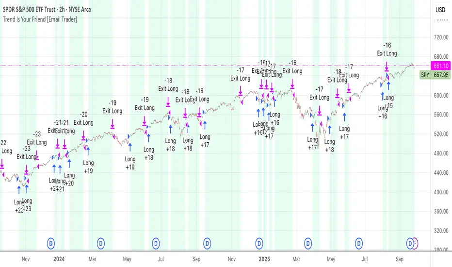
TrendIsYourFriend Strategy (SPY,IWM,VYM,XLK,SPXL,BTC,GOLD,VT...)Personal disclaimer
Don’t trust this strategy. Don’t trust any other model either just because of its author or a backtest curve. Overfitting is an easy trap, and beginners often fall into it. This script isn’t meant to impress you. It’s meant to survive reality. If it does, maybe it will raise questions and you’ll remember it.
Legal disclaimer
Educational purposes only. Not financial advice. Past performance is not indicative of future results.
Strategy description
Long-only, trend-based logic with two entry types (trend continuation or excess-move reversion), dynamic stop-losses, and a VIX filter to avoid turbulent markets.
Minimal number of parameters with enough trades to support robustness.
For backtest, each trade is sized at $10,000 flat (no compounding, to focus on raw model quality and the regularity of its results over time).
Fees = $0 (neutral choice, as brokers differ).
Slippage = $0, deliberate choice: most entries occur on higher timeframes, and some assets start their history on charts at very low prices, which would otherwise distort results.
What makes this script original
Beyond a classical trend calculation, both excess-move entries and dynamic stop-loss exits also rely on trend logic. Except for the VIX filter, everything comes from trend functions, with very few parameters.
Pre-configurations are fixed in the code, allowing sincere performance tracking across a dozen cases over the medium to long term.
Allowed
SPY (ARCA) — 2-hour chart: S&P 500 ETF, most liquid equity benchmark
IWM (ARCA) — Daily chart: Russell 2000 ETF, US small caps
VYM (ARCA) — Daily chart: Vanguard High Dividend Yield ETF
XLK (ARCA) — Daily chart: Technology Select Sector SPDR
SPXL (ARCA) — Daily chart: 3× leveraged S&P 500 ETF
BTCUSD (COINBASE) — 4-hour chart: Bitcoin vs USD
GOLD (TVC) — Daily chart: Gold spot price
VT (ARCA) — Daily chart: Vanguard Total World Stock ETF
PG (NYSE) — Daily chart: Procter & Gamble Co.
CQQQ (ARCA) — Daily chart: Invesco China Technology ETF
EWC (ARCA) — Daily chart: iShares MSCI Canada ETF
EWJ (ARCA) — Daily chart: iShares MSCI Japan ETF
How to use and form an opinion on it
Works only on the pairs above.
Feel free to modify the input parameters (slippage, fees, order size, margins, …) to see how the model behaves under your own conditions
Compare it with a simple Buy & Hold (requires an order size of 100% equity).
You may also want to look at its time-in-market — the share of time your capital is actually at risk.
Finally, let me INSIST on this : let it run live for months before forming an opinion!
Share your thoughts in the comments 🚀 if you’d like to discuss its live performance.
THE BATATAH SAUCE BTC.PERP TRADING STRAT12hr hour is the sweet spot
great profit factor
decent risk management avg losing (back tested for 5 yrs and does alright till even 2018)trade 8.21% vs avg winning 174.87% (back tested for 5 yrs and does alright since even start2018)
Its alright on daily as well as 6hr but lower just gets more noisy

Signalgo Strategy ISignalgo Strategy I: Technical Overview
Signalgo Strategy I is a systematically engineered TradingView strategy script designed to automate, test, and manage trend-following trades using multi-timeframe price/volume logic, volatility-based targets, and multi-layered exit management. This summary covers its operational structure, user inputs, entry and exit methodology, unique technical features, and practical application.
Core Logic and Workflow
Multi-Timeframe Data Synthesis
User-Defined Timeframe: The user chooses a timeframe (e.g., 1H, 4H, 1D, etc.), on which all strategy signals are based.
Cross-Timeframe Inputs: The strategy imports closing price, volume, and Average True Range (ATR) for the selected interval, independently from the chart’s native timeframe, enabling robust multi-timeframe analysis.
Price Change & Volume Ratio: It calculates the percent change of price per bar and computes a volume ratio by comparing current volume to its 20-bar moving average—enabling detection of true “event” moves vs. normal market noise.
Hype Filtering
Anti-Hype Mechanism: An entry is automatically filtered out if abnormal high volume occurs without corresponding price movement, commonly observed during manipulation or announcement periods. This helps isolate genuine market-driven momentum.
User Inputs
Select Timeframe: Choose which interval drives signal generation.
Backtest Start Date: Specify from which date historical signals are included in the strategy (for precise backtests).
Take-Profit/Stop-Loss Configuration: Internally, risk levels are set as multiples of ATR and allow for three discrete profit targets.
Entry Logic
Trade Signal Criteria:
Price change magnitude in the current bar must exceed a fixed sensitivity threshold.
Volume for the bar must be significantly elevated compared to average, indicating meaningful participation.
Anti-hype check must not be triggered.
Bullish/Bearish Determination: If all conditions are met and price change direction is positive, a long signal triggers. If negative, a short signal triggers.
Signal Debouncing: Ensures a signal triggers only when a new condition emerges, avoiding duplicate entries on flat or choppy bars.
State Management: The script tracks whether an active long or short is open to avoid overlapping entries and to facilitate clean reversals.
Exit Strategy
Take-Profits: Three distinct profit targets (TP1, TP2, TP3) are calculated as fixed multiples of the ATR-based stop loss, adapting dynamically to volatility.
Reversals: If a buy signal appears while a short is open (or vice versa), the existing trade is closed and reversed in a single step.
Time-Based Exit: If, 49 bars after entry, the trade is in-profit but hasn’t reached TP1, it exits to avoid stagnation risk.
Adverse Move Exit: The position is force-closed if it suffers a 10% reversal from entry, acting as a catastrophic stop.
Visual Feedback: Each TP/SL/exit is plotted as a clear, color-coded line on the chart; no hidden logic is used.
Alerts: Built-in TradingView alert conditions allow automated notification for both entries and strategic exits.
Distinguishing Features vs. Traditional MA Strategies
Event-Based, Not Just Slope-Based: While classic moving average strategies enter trades on MA crossovers or slope changes, Signalgo Strategy I demands high-magnitude price and volume confirmation on the chosen timeframe.
Volume Filtering: Very few MA strategies independently filter for meaningful volume spikes.
Real Market Event Focus: The anti-hype filter differentiates organic market trends from manipulated “high-volume, no-move” sessions.
Three-Layer Exit Logic: Instead of a single trailing stop or fixed RR, this script manages three profit targets, time-based closures, and hard adverse thresholds.
Multi-Timeframe, Not Chart-Dependent: The “main” analytical interval can be set independently from the current chart, allowing for in-depth cross-timeframe backtests and system runs.
Reversal Handling: Automatic handling of signal reversals closes and flips positions precisely, reducing slippage and manual error.
Persistent State Tracking: Maintains variables tracking entry price, trade status, and target/stop levels independently of chart context.
Trading Application
Strategy Sandbox: Designed for robust backtesting, allowing users to simulate performance across historical data for any major asset or interval.
Active Risk Management: Trades are consistently managed for both fixed interval “stall” and significant loss, not just via trailing stops or fixed-day closes.
Alert Driven: Can power algorithmic trading bots or notify discretionary traders the moment a qualifying market event occurs.

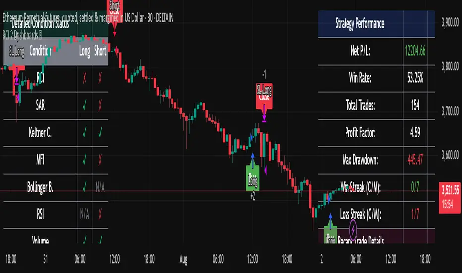
RCI 2 Dashboards ✅ Strategy: RCI 2 Dashboards BY Sonu JAIN
This advanced strategy is built around the Rank Correlation Index (RCI), a unique momentum oscillator, and combines it with a comprehensive suite of powerful indicators to identify high-probability trading opportunities. The strategy’s core strength lies in its ability to filter signals using up to 12 different conditions for both long and short trades.
To make the decision-making process clear and intuitive, the strategy features two dynamic, customizable dashboards right on your chart. The first dashboard gives you a live, detailed breakdown of which conditions are met, while the second provides a real-time overview of the strategy’s performance.
How It Works
The strategy generates entry signals based on RCI crossovers and crossunders. These signals are then filtered by a customizable combination of other indicators to confirm the trade.
Long Entry:
The RCI crosses over its moving average.
All enabled long-side filters are met.
Short Entry:
The RCI crosses under its moving average.
All enabled short-side filters are met.
Key Features
RCI Crossover Logic: The core of the strategy is an RCI crossover/crossunder with a customizable moving average (MA). You can choose from SMA, EMA, SMMA (RMA), WMA, or VWMA.
12 Optional Filters: This strategy goes far beyond a simple RCI signal. You can enable or disable a wide range of filters to refine your entries. These include:
Trend: Supertrend, Parabolic SAR (SAR), and Vortex Indicator.
Volatility: Keltner Channels (KC) and Bollinger Bands (BB).
Momentum: Woodies CCI, Money Flow Index (MFI), and Relative Strength Index (RSI).
Volume: On-Balance Volume (OBV) and simple Volume analysis.
Directional Strength: Average Directional Index (ADX).
Timing: A time-of-day filter to trade only during specific market hours.
Dual Dashboards:
Detailed Condition Dashboard: This dashboard shows you exactly which of the 12 filters are currently met with a simple ✓ or ✗. This provides instant clarity on why a trade is or isn't being considered.
Performance Dashboard: This dashboard displays key performance metrics in real-time, including net profit, win rate, profit factor, max drawdown, and current/max winning and losing streaks. It also provides details on the most recent trade, such as entry, stop-loss, and exit prices.
Customizable Stop Loss: The strategy includes a fixed percentage-based stop loss for both long and short positions, which you can easily configure in the settings.
Trade Direction Control: You can choose to trade "Long Only," "Short Only," or "Long & Short," giving you complete control over your trading bias.
This strategy is a powerful tool for traders who want to build a robust, multi-filtered system. The included dashboards make it an excellent educational tool for understanding how different indicators work together to form a complete trading plan. You can use it to backtest and optimize your own unique combination of indicators to find the perfect setup for your market and timeframe.
Auto Intelligence Selective Moving Average(AI/MA)# 🤖 Auto Intelligence Moving Average Strategy (AI/MA)
**AI/MA** is a state-adaptive moving average crossover strategy designed to **maximize returns from golden cross / death cross logic** by intelligently switching between different MA types and parameters based on market conditions.
---
## 🎯 Objective
To build a moving average crossover strategy that:
- **Adapts dynamically** to market regimes (trend vs range, rising vs falling)
- **Switches intelligently** between SMA, EMA, RMA, and HMA
- **Maximizes cumulative return** under realistic backtesting
---
## 🧪 materials amd methods
- **MA Types Considered**: SMA, EMA, RMA, HMA
- **Parameter Ranges**: Periods from 5 to 40
- **Market Conditions Classification**:
- Based on the slope of a central SMA(20) line
- And the relative position of price to the central line
- Resulting in 4 regimes: A (Bull), B (Pullback), C (Rebound), D (Bear)
- **Optimization Dataset**:
- **Bybit BTCUSDT.P**
- **1-hour candles**
- **2024 full-year**
- **Search Process**:
- **Random search**: 200 parameter combinations
- Evaluated by:
- `Cumulative PnL`
- `Sharpe Ratio`
- `Max Drawdown`
- `R² of linear regression on cumulative PnL`
- **Implementation**:
- Optimization performed in **Python (Pandas + Matplotlib + Optuna-like logic)**
- Final parameters ported to **Pine Script (v5)** for TradingView backtesting
---
## 📈 Performance Highlights (on optimization set)
| Timeframe | Return (%) | Notes |
|-----------|------------|----------------------------|
| 6H | +1731% | Strongest performance |
| 1D | +1691% | Excellent trend capture |
| 12H | +1438% | Balance of trend/range |
| 5min | +27.3% | Even survives scalping |
| 1min | +9.34% | Robust against noise |
- Leverage: 100x
- Position size: 100%
- Fees: 0.055%
- Margin calls: **none** 🎯
---
## 🛠 Technology Stack
- `Python` for data handling and optimization
- `Pine Script v5` for implementation and visualization
- Fully state-aware strategy, modular and extendable
---
## ✨ Final Words
This strategy is **not curve-fitted**, **not over-parameterized**, and has been validated across multiple timeframes. If you're a fan of dynamic, intelligent technical systems, feel free to use and expand it.
💡 The future of simple-yet-smart trading begins here.

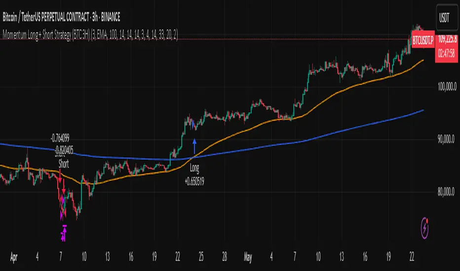
Momentum Long + Short Strategy (BTC 3H)Momentum Long + Short Strategy (BTC 3H)
🔍 How It Works, Step by Step
Detect the Trend (📈/📉)
Calculate two moving averages (100-period and 500-period), either EMA or SMA.
For longs, we require MA100 > MA500 (uptrend).
For shorts, we block entries if MA100 exceeds MA500 by more than a set percentage (to avoid fading a powerful uptrend).
Apply Momentum Filters (⚡️)
RSI Filter: Measures recent strength—only allow longs when RSI crosses above its smoothed average, and shorts when RSI dips below the oversold threshold.
ADX Filter: Gauges trend strength—ensures we only enter when a meaningful trend exists (optional).
ATR Filter: Confirms volatility—avoids choppy, low-volatility conditions by requiring ATR to exceed its smoothed value (optional).
Confirm Entry Conditions (✅)
Long Entry:
Price is above both MAs
Trend alignment & optional filters pass ✅
Short Entry:
Price is below both MAs and below the lower Bollinger Band
RSI is sufficiently oversold
Trend-blocker & ATR filter pass ✅
Position Sizing & Risk (💰)
Each trade uses 100 % of account equity by default.
One pyramid addition allowed, so you can scale in if the move continues.
Commission and slippage assumptions built in for realistic backtests.
Stops & Exits (🛑)
Long Stop-Loss: e.g. 3 % below entry.
Long Auto-Exit: If price falls back under the 500-period MA.
Short Stop-Loss: e.g. 3 % above entry.
Short Take-Profit: e.g. 4 % below entry.
🎨 Why It’s Powerful & Customizable
Modular Filters: Turn on/off RSI, ADX, ATR filters to suit different market regimes.
Adjustable Thresholds: Fine-tune stop-loss %, take-profit %, RSI lengths, MA gaps and more.
Multi-Timeframe Potential: Although coded for 3 h BTC, you can adapt it to stocks, forex or other cryptos—just recalibrate!
Backtest Fine-Tuned: Default settings were optimized via backtesting on historical BTC data—but they’re not guarantees of future performance.
⚠️ Warning & Disclaimer
This strategy is for educational purposes only and designed for a toy fund. Crypto markets are highly volatile—you can lose 100 % of your capital. It is not a predictive “holy grail” but a rules-based framework using past data. The parameters have been fine-tuned on historical data and are not valid for future trades without fresh calibration. Always practice with paper-trading first, use proper risk management, and do your own research before risking real money. 🚨🔒
Good luck exploring and experimenting! 🚀📊
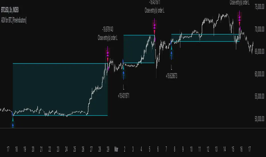
ADX for BTC [PineIndicators]The ADX Strategy for BTC is a trend-following system that uses the Average Directional Index (ADX) to determine market strength and momentum shifts. Designed for Bitcoin trading, this strategy applies a customizable ADX threshold to confirm trend signals and optionally filters entries using a Simple Moving Average (SMA). The system features automated entry and exit conditions, dynamic trade visualization, and built-in trade tracking for historical performance analysis.
⚙️ Core Strategy Components
1️⃣ Average Directional Index (ADX) Calculation
The ADX indicator measures trend strength without indicating direction. It is derived from the Positive Directional Movement (+DI) and Negative Directional Movement (-DI):
+DI (Positive Directional Index): Measures upward price movement.
-DI (Negative Directional Index): Measures downward price movement.
ADX Value: Higher values indicate stronger trends, regardless of direction.
This strategy uses a default ADX length of 14 to smooth out short-term fluctuations while detecting sustainable trends.
2️⃣ SMA Filter (Optional Trend Confirmation)
The strategy includes a 200-period SMA filter to validate trend direction before entering trades. If enabled:
✅ Long Entry is only allowed when price is above a long-term SMA multiplier (5x the standard SMA length).
✅ If disabled, the strategy only considers the ADX crossover threshold for trade entries.
This filter helps reduce entries in sideways or weak-trend conditions, improving signal reliability.
📌 Trade Logic & Conditions
🔹 Long Entry Conditions
A buy signal is triggered when:
✅ ADX crosses above the threshold (default = 14), indicating a strengthening trend.
✅ (If SMA filter is enabled) Price is above the long-term SMA multiplier.
🔻 Exit Conditions
A position is closed when:
✅ ADX crosses below the stop threshold (default = 45), signaling trend weakening.
By adjusting the entry and exit ADX levels, traders can fine-tune sensitivity to trend changes.
📏 Trade Visualization & Tracking
Trade Markers
"Buy" label (▲) appears when a long position is opened.
"Close" label (▼) appears when a position is exited.
Trade History Boxes
Green if a trade is profitable.
Red if a trade closes at a loss.
Trend Tracking Lines
Horizontal lines mark entry and exit prices.
A filled trade box visually represents trade duration and profitability.
These elements provide clear visual insights into trade execution and performance.
⚡ How to Use This Strategy
1️⃣ Apply the script to a BTC chart in TradingView.
2️⃣ Adjust ADX entry/exit levels based on trend sensitivity.
3️⃣ Enable or disable the SMA filter for trend confirmation.
4️⃣ Backtest performance to analyze historical trade execution.
5️⃣ Monitor trade markers and history boxes for real-time trend insights.
This strategy is designed for trend traders looking to capture high-momentum market conditions while filtering out weak trends.
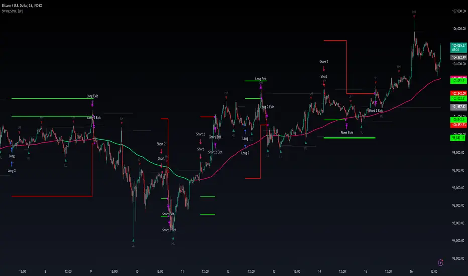
Swing High/Low Pivots Strategy [LV]The Swing High/Low Pivots Strategy was developed as a counter-momentum trading tool.
The strategy is suitable for any market and the default values used in the input settings menu are set for Bitcoin (best on 15min). These values, expressed in minimum ticks (or pips if symbol is Forex) make this tool perfectly adaptable to every symbol and/or timeframe.
Check tooltips in the settings menu for more details about every user input.
STRTEGY ENTRY & EXIT MECHANISMS:
Trades Entry based on the detection of swing highs and lows for short and long entries respectively, validated by:
- Limit orders placed after each new pivot level confirmation
- Moving averages trend filter (if enabled)
- No active trade currently open
Trades Exit when the price reaches take-profit or stop-loss level as defined in the settings menu. A double entry/second take-profit level can be enabled for partial exits, with dynamic stop-loss adjustment for the remaining position.
Enhanced Trade Precision:
By limiting entries to confirmed swing high (HH, LH) or swing low (HL, LL) pivot points, the strategy ensures that trades occur at levels of significant price reversals. This precision reduces the likelihood of entering trades in the midst of a trend or during uncertain price action.
Risk Management Optimization:
The strategy incorporates clearly defined stop-loss (SL) and take-profit (TP) levels derived from the pivot points. This structured approach minimizes potential losses while locking in profits, which is critical for consistent performance in volatile markets.
Trend Filtering for Better Entry:
The use of a configurable moving average filter adds a layer of trend validation. This prevents entering trades against the dominant market trend, increasing the probability of success for each trade.
Avoidance of Noise:
The lookback period (length parameter) confirms pivots only after a set number of bars, effectively filtering out market noise and ensuring that entries are based on reliable, well-defined price movements.
Adaptability Across Markets:
The strategy is versatile and can be applied across different markets (Forex, stocks, crypto) due to its dynamic use of ticks and pips converters. It adapts seamlessly to varying price scales and asset types.
Dual Quantity Entries:
The original and optionnal double-entry mechanism allows traders to capture both short-term and extended profits by scaling out of positions. This adaptive approach caters to varying risk appetites and market conditions.
Clear Visualization:
The plotted pivot points, entry limits, SL, and TP levels provide visual clarity, making it easy for traders to track the strategy's behavior and make informed decisions.
Automated Execution with Alerts:
Integrated alerts for both entries and exits ensure timely actions without the need for constant market monitoring, enhancing efficiency. Configurable alert messages are suitable for API use.
Any feedback, comments, or suggestions for improvement are always welcome.
Hope you enjoy!
HFT V.2 EnhancedTitle: HFT V.2 Enhanced - ATR Dynamic Stop-Loss & Take-Profit
Description:
The HFT V.2 Enhanced strategy is designed for high-frequency trading with dynamic trade management and robust entry/exit logic. This strategy uses simple moving averages (SMA) for trend identification and the relative strength index (RSI) for momentum confirmation. In this enhanced version, the strategy also incorporates dynamic stop-loss and take-profit levels based on the Average True Range (ATR), offering better adaptability to market volatility.
Features:
Moving Average Crossover: Uses a fast and slow SMA to capture trend reversals and generate trade entries.
RSI Confirmation: Ensures momentum is in the direction of the trade by incorporating the RSI threshold for both long and short entries.
Dynamic Stop-Loss and Take-Profit: Stop-loss and take-profit levels are calculated based on the ATR, allowing the strategy to adjust its exit points according to market volatility. This helps manage risk more effectively and capture larger trends.
Auto-Close Opposing Positions: Automatically closes any open long positions when a short entry is triggered, and vice versa.
Once-Per-Bar Execution: Ensures that a position is entered only once per bar, avoiding multiple trades within the same bar.
Parameters:
Fast MA Length: Defines the length of the fast-moving average.
Slow MA Length: Defines the length of the slow-moving average.
RSI Length: Sets the period for the RSI indicator.
RSI Threshold: Controls the RSI level for confirming momentum (50 by default).
ATR Length: Determines the period for the ATR calculation.
ATR Multiplier for Stop-Loss/Take-Profit: Adjusts the sensitivity of the stop-loss and take-profit levels based on ATR.
How it Works:
Long Entry: The strategy opens a long trade when the fast SMA crosses above the slow SMA, and the RSI is above the user-defined threshold. A dynamic stop-loss is placed below the entry price, and a take-profit target is set based on ATR.
Short Entry: The strategy opens a short trade when the fast SMA crosses below the slow SMA, and the RSI is below the inverse threshold. A stop-loss is placed above the entry price, and a take-profit target is set using ATR.
Risk Management: The strategy adapts to changing market conditions by dynamically adjusting its stop-loss and take-profit levels, ensuring it remains responsive to market volatility.
This script is ideal for traders looking for a high-frequency strategy with advanced trade management, including dynamic exits and volatility-based risk management.
Disclaimer: Always backtest and optimize the parameters to fit your trading style and risk tolerance before using the strategy in live trading.

Rsi Long-Term Strategy [15min]Hello, I would like to present to you The "RSI Long-Term Strategy" for 15min tf
The "RSI Long-Term Strategy " is designed for traders who prefer a combination of momentum and trend-following techniques. The strategy focuses on entering long positions during significant market corrections within an overall uptrend, confirmed by both RSI and volume. The use of long-term SMAs ensures that trades are made in line with the broader market trend. The stop-loss feature provides risk management by limiting losses on trades that do not perform as expected. This strategy is particularly well-suited for longer-term traders who monitor 15-minute charts but look for substantial trend reversals or continuations.
Indicators and Parameters:
Relative Strength Index (RSI):
- The RSI is calculated using a 10-period length. It measures the magnitude of recent price changes to evaluate overbought or oversold conditions. The script defines oversold conditions when the RSI is at or below 30 and overbought conditions when the RSI is at or above 70.
Volume Condition:
-The strategy incorporates a volume condition where the current volume must be greater than 2.5 times the 20-period moving average of volume. This is used to confirm the strength of the price movement.
Simple Moving Averages (SMA):
- The strategy uses two SMAs: SMA1 with a length of 250 periods and SMA2 with a length of 500 periods. These SMAs help identify long-term trends and generate signals based on their crossover.
Strategy Logic:
Entry Logic:
A long position is initiated when all the following conditions are met:
The RSI indicates an oversold condition (RSI ≤ 30).
SMA1 is above SMA2, indicating an uptrend.
The volume condition is satisfied, confirming the strength of the signal.
Exit Logic:
The strategy closes the long position when SMA1 crosses under SMA2, signaling a potential end of the uptrend (a "Death Cross").
Stop-Loss:
A stop-loss is set at 5% below the entry price to manage risk and limit potential losses.
Buy and sell signals are highlighted with circles below or above bars:
Green Circle : Buy signal when RSI is oversold, SMA1 > SMA2, and the volume condition is met.
Red Circle : Sell signal when RSI is overbought, SMA1 < SMA2, and the volume condition is met.
Black Cross: "Death Cross" when SMA1 crosses under SMA2, indicating a potential bearish signal.
to determine the level of stop loss and target point I used a piece of code by RafaelZioni, here is the script from which a piece of code was taken
I hope the strategy will be helpful, as always, best regards and safe trades
;)
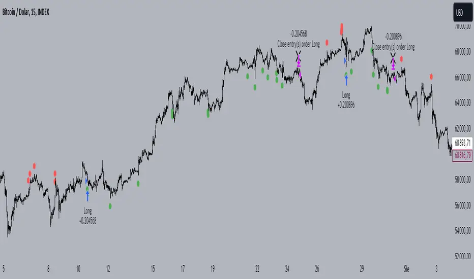
Quatro SMA Strategy [4h]Hello, I would like to present to you The "Quatro SMA" strategy
Strategy is based on four simple moving averages of different lengths and monitoring trading volume. The key idea is to identify strong market trends by comparing short-term moving averages with the long-term SMA. The strategy generates buy signals when all short-term SMAs are above the SMA(200) and the volume confirms the strength of the move. Similarly, sell signals are generated when all short-term SMAs are below the SMA(200), and the volume is sufficiently high.
The strategy manages risk by applying a stop loss and three different Take Profit levels (TP1, TP2, TP3), with varying percentages of the position closed at each level.
Each Take Profit level is triggered at a specific percentage gain, with the position being closed gradually depending on the achieved targets. The percentage of the position closed at each TP level is also defined by the user.
Indicators and Parameters:
Simple Moving Averages (SMA):
The script utilizes four simple moving averages with different lengths (4, 16, 32, 200). The first three SMAs (SMA1, SMA2, SMA3) are used to determine the trend direction, while the fourth SMA (with a length of 200) serves as a support/resistance line.
Volume:
The script monitors trading volume and checks if the current volume exceeds 2.5 times the average volume of the last 40 candles. High volume is considered as confirmation of trend strength.
Entry Conditions:
- Long Position: Triggered when SMA1 > SMA2 > SMA3, the closing price is above SMA(200), and the volume condition is met.
- Short Position: Triggered when SMA1 < SMA2 < SMA3, the closing price is below SMA(200), and the volume condition is met.
Exit Conditions:
- Long Position: Closed when SMA1 < SMA2 < SMA3 and the closing price is above SMA(200).
- Short Position: Closed when SMA1 > SMA2 > SMA3 and the closing price is below SMA(200).
to determine the level of stop loss and target point I used a piece of code by RafaelZioni, here is the script from which a piece of code was taken
I hope the strategy will be helpful, as always, best regards and safe trades
;)