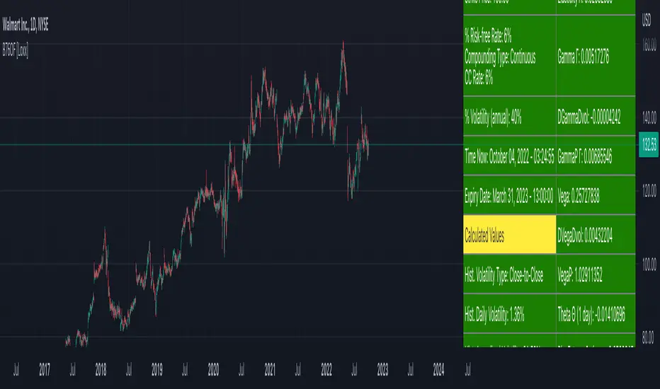
Black-76 Options on Futures [Loxx]Black-76 Options on Futures is an adaptation of the Black-Scholes-Merton Option Pricing Model including Analytical Greeks and implied volatility calculations. The following information is an excerpt from Espen Gaarder Haug's book "Option Pricing Formulas". This version is to price Options on Futures. The options sensitivities (Greeks) are the partial derivatives of the Black-Scholes-Merton ( BSM ) formula. Analytical Greeks for our purposes here are broken down into various categories:
Delta Greeks: Delta, DDeltaDvol, Elasticity
Gamma Greeks: Gamma, GammaP, DGammaDvol, Speed
Vega Greeks: Vega , DVegaDvol/Vomma, VegaP
Theta Greeks: Theta
Rate/Carry Greeks: Rho futures option
Probability Greeks: StrikeDelta, Risk Neutral Density
(See the code for more details)
Black-Scholes-Merton Option Pricing
The Black-Scholes-Merton model can be "generalized" by incorporating a cost-of-carry rate b. This model can be used to price European options on stocks, stocks paying a continuous dividend yield, options on futures , and currency options:
c = S * e^((b - r) * T) * N(d1) - X * e^(-r * T) * N(d2)
p = X * e^(-r * T) * N(-d2) - S * e^((b - r) * T) * N(-d1)
where
d1 = (log(S / X) + (b + v^2 / 2) * T) / (v * T^0.5)
d2 = d1 - v * T^0.5
b = r ... gives the Black and Scholes (1973) stock option model.
b = r — q ... gives the Merton (1973) stock option model with continuous dividend yield q.
b = 0 ... gives the Black (1976) futures option model. <== this is the one used for this indicator!
b = 0 and r = 0 ... gives the Asay (1982) margined futures option model.
b = r — rf ... gives the Garman and Kohlhagen (1983) currency option model.
Inputs
S = Stock price.
X = Strike price of option.
T = Time to expiration in years.
r = Risk-free rate
d = dividend yield
v = Volatility of the underlying asset price
cnd (x) = The cumulative normal distribution function
nd(x) = The standard normal density function
convertingToCCRate(r, cmp ) = Rate compounder
gImpliedVolatilityNR(string CallPutFlag, float S, float x, float T, float r, float b, float cm , float epsilon) = Implied volatility via Newton Raphson
gBlackScholesImpVolBisection(string CallPutFlag, float S, float x, float T, float r, float b, float cm ) = implied volatility via bisection
Implied Volatility: The Bisection Method
The Newton-Raphson method requires knowledge of the partial derivative of the option pricing formula with respect to volatility ( vega ) when searching for the implied volatility . For some options (exotic and American options in particular), vega is not known analytically. The bisection method is an even simpler method to estimate implied volatility when vega is unknown. The bisection method requires two initial volatility estimates (seed values):
1. A "low" estimate of the implied volatility , al, corresponding to an option value, CL
2. A "high" volatility estimate, aH, corresponding to an option value, CH
The option market price, Cm , lies between CL and cH . The bisection estimate is given as the linear interpolation between the two estimates:
v(i + 1) = v(L) + (c(m) - c(L)) * (v(H) - v(L)) / (c(H) - c(L))
Replace v(L) with v(i + 1) if c(v(i + 1)) < c(m), or else replace v(H) with v(i + 1) if c(v(i + 1)) > c(m) until |c(m) - c(v(i + 1))| <= E, at which point v(i + 1) is the implied volatility and E is the desired degree of accuracy.
Implied Volatility: Newton-Raphson Method
The Newton-Raphson method is an efficient way to find the implied volatility of an option contract. It is nothing more than a simple iteration technique for solving one-dimensional nonlinear equations (any introductory textbook in calculus will offer an intuitive explanation). The method seldom uses more than two to three iterations before it converges to the implied volatility . Let
v(i + 1) = v(i) + (c(v(i)) - c(m)) / (dc / dv (i))
until |c(m) - c(v(i + 1))| <= E at which point v(i + 1) is the implied volatility , E is the desired degree of accuracy, c(m) is the market price of the option, and dc/ dv (i) is the vega of the option evaluaated at v(i) (the sensitivity of the option value for a small change in volatility ).
Things to know
Only works on the daily timeframe and for the current source price.
You can adjust the text size to fit the screen
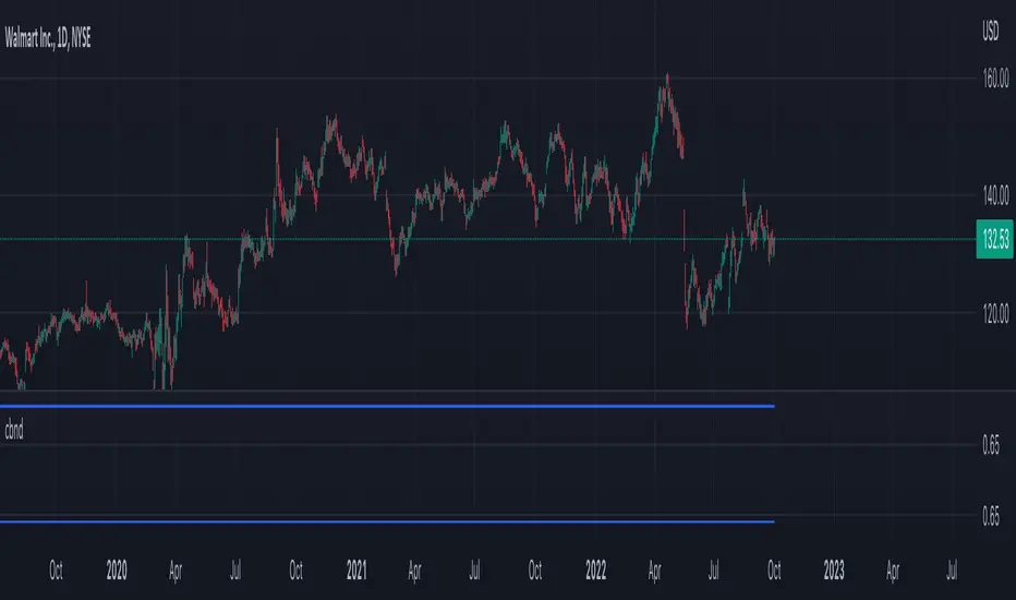
Cumulativenormaldistribution
cbndLibrary "cbnd"
Description:
A standalone Cumulative Bivariate Normal Distribution (CBND) functions that do not require any external libraries.
This includes 3 different CBND calculations: Drezner(1978), Drezner and Wesolowsky (1990), and Genz (2004)
Comments:
The standardized cumulative normal distribution function returns the probability that one random
variable is less than a and that a second random variable is less than b when the correlation
between the two variables is p. Since no closed-form solution exists for the bivariate cumulative
normal distribution, we present three approximations. The first one is the well-known
Drezner (1978) algorithm. The second one is the more efficient Drezner and Wesolowsky (1990)
algorithm. The third is the Genz (2004) algorithm, which is the most accurate one and therefore
our recommended algorithm. West (2005b) and Agca and Chance (2003) discuss the speed and
accuracy of bivariate normal distribution approximations for use in option pricing in
ore detail.
Reference:
The Complete Guide to Option Pricing Formulas, 2nd ed. (Espen Gaarder Haug)
CBND1(A, b, rho)
Returns the Cumulative Bivariate Normal Distribution (CBND) using Drezner 1978 Algorithm
Parameters:
A : float,
b : float,
rho : float,
Returns: float.
CBND2(A, b, rho)
Returns the Cumulative Bivariate Normal Distribution (CBND) using Drezner and Wesolowsky (1990) function
Parameters:
A : float,
b : float,
rho : float,
Returns: float.
CBND3(x, y, rho)
Returns the Cumulative Bivariate Normal Distribution (CBND) using Genz (2004) algorithm (this is the preferred method)
Parameters:
x : float,
y : float,
rho : float,
Returns: float.
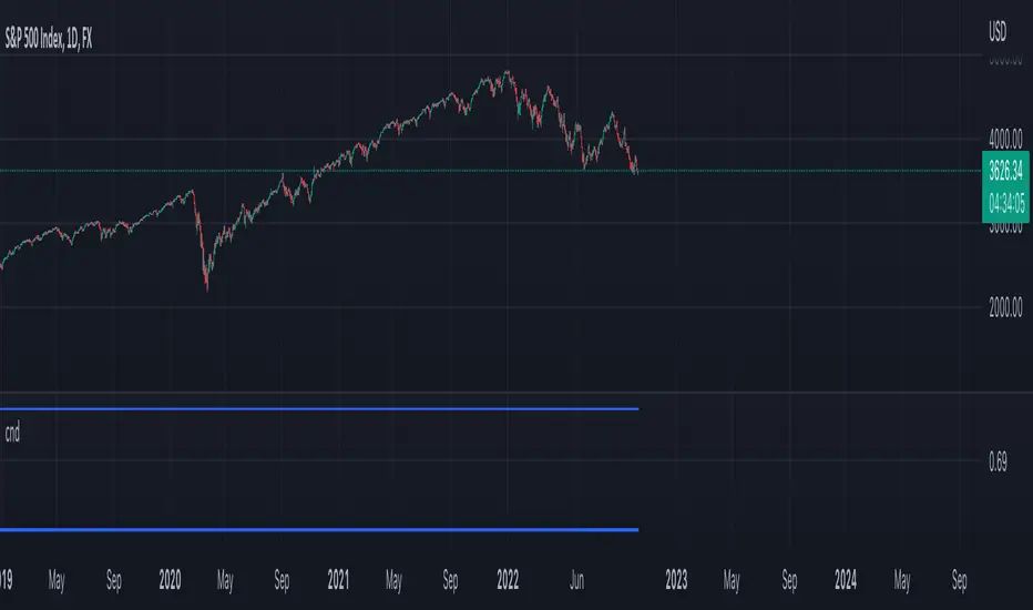
cndLibrary "cnd"
Cumulative Normal Distribution
CND1(x)
Returns the Cumulative Normal Distribution (CND) using the Hart (1968) method. (preferred method, 14-18 decimal accuracy)
Parameters:
x : float,
Returns: float.
CND2(x)
Returns the Cumulative Normal Distribution (CND) using the Abromowitz and Stegun (1974) Polynomial Approximation.
Parameters:
x : float,
Returns: float.
CND3(x)
Returns the Cumulative Normal Distribution (CND) using Newton-Cotes method, Boole’s rule
Parameters:
x : float,
Returns: float.
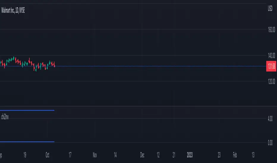
chi2InvLibrary "chi2Inv"
chi2Inv(p, n)
Returns the inverse cumulative distribution function (icdf) of the chi-square distribution with degrees of freedom nu, evaluated at the probability values in p. Goldstein approximation
Parameters:
p : float, probability
n : float, degress of freedom source.
Returns: float.