RunRox - Pairs Strategy🧬 Pairs Strategy is a new indicator by RunRox included in our premium subscription.
It is a specialized tool for trading pairs, built around working with two correlated instruments at the same time.
The indicator is designed specifically for pair trading logic: it helps track the relationship between two assets, identify statistical deviations, and generate signals for opening and managing long/short combinations on both legs of the pair.
Below in this description I will go through the core functions of the indicator and the main concepts behind the strategy so you can clearly understand how to apply it in your trading.
📌 CONCEPT
The core idea of pair trading is to find and trade correlated instruments that usually move in a similar way.
When these two assets temporarily diverge from each other, a trading opportunity appears.
In such moments, the relatively overvalued asset is sold (short leg), and the relatively undervalued asset is bought (long leg).
When the spread between them narrows and both instruments revert back toward their typical relationship (mean), the position is closed and the trader captures the profit from this convergence.
In practice, one leg of the pair can end up in a loss while the other generates a larger profit.
Due to the difference in performance between the two assets, the combined result of the pair trade can still be positive.
✅ KEY FEATURES:
2 deviation types (Z-Score and S-Score)
Invert signals mode
Hedge Coefficient (position size balancing between both legs)
6 hedge modes
Entries based on Score or RSI
Extra entries based on Score or Spread
Stop Loss
Take Profit
RSI Filter
RSI Pivot Mode
Built-in Backtester Strategy
Lower Timeframe Backtester Strategy
Live trade panel for current position
Equity curve chart
21 performance metrics in the backtester
2 alert types
*And many more fine-tuning options for pair trading
🔗 SCORE
Score is the core deviation metric between the two assets in the pair.
For example, if you are trading ETHUSDT/BTCUSDT, the indicator analyzes the relationship ETH/BTC, and when one leg temporarily diverges from the other, this difference is reflected in the Score value.
In other words, Score shows how much the current spread between the two instruments deviates from its typical state and is used as the main signal source for pair entries and exits.
In the screenshot above you can see how Score looks in our indicator.
Depending on how large the difference is between the two assets, the Score value can move in a range from −N to +N
When Score is in the −N zone, this is a 🟢 long zone for the first asset and a short zone for the second.
Using the ETH/BTC example: when Score is deeply negative, you open a long on ETH and a short on BTC at the same time, then close both legs when Score returns back to the 0 zone (balance between the two assets).
When Score is in the +N zone, this is a 🔴 short zone for the first asset and a long zone for the second.
In the same ETH/BTC example: when Score is strongly positive, you short ETH and long BTC, and again close both positions when Score comes back to the neutral 0 zone.
☯️ Z/S SCORE
Inside the indicator we added two different formulas for calculating the spread between the two legs of the pair: Z-Score and S-Score.
These approaches measure deviation in different ways and can produce slightly different signals depending on the chosen pair and its behavior.
This allows you to switch between Z-Score and S-Score and choose the method that gives more stable and cleaner signals for your specific instruments.
As you can see in the screenshot above, we used the same pair but applied different Score types to measure the spread and deviation from the norm.
🟣 Z-Score – generated 9 entry signals .
It reacts to price fluctuations more smoothly and usually stays within a range of approximately −8 to +8 .
🟠 S-Score – generated 5 entry signals .
It reacts to price changes more aggressively and produces wider deviations, often reaching −15 to +15 .
This gives traders the choice between a more sensitive but smoother model (Z-Score) and a more selective, stronger-deviation model (S-Score)
⁉️ HOW DOES THE STRATEGY WORK
Here is a basic example of how you can trade this pair trading strategy using our indicator and its signals.
In the classic approach the trade consists of one initial entry and several scale-ins (averaging) if the spread continues to move against the position.
The first entry is opened when Score reaches a standard deviation of −2 or +2.
If price does not revert to the mean and moves further against the position so that Score expands to −3 or +3, the strategy performs the first scale-in.
If Score extends to −4 or +4, a second scale-in is added.
If the spread grows even more and Score reaches −5 or +5, a third scale-in is executed.
In our indicator the number of averaging steps can be up to 4 scale-ins .
After that the position waits until Score returns back to the 0 level , where the whole pair position is closed.
This is the standard model of classical pair trading.
However there are many variations:
using Stop Loss and Take Profit,
exiting earlier or later than the 0 zone,
scaling in not by Score but by Spread, since Score is not linear while Spread is linear,
entering when RSI on both tickers shows opposite extremes, for example RSI 20 on one asset and RSI 80 on the other, and so on.
The number of possible trading styles for this strategy is very large.
We designed the indicator to cover as many of these variations as possible and added flexible tools so you can build your own pair trading logic on top of it.
Below is an example of a classic pair trade with two entries: one main entry and one extra entry (scale-in) .
The pair SUIUSDT / PENGUUSDT shows a high correlation, and on one of the trades the sequence looked like this:
A −2 Score deviation occurred into the long zone and triggered the Main Entry .
🔹 Main Entry
Long SUIUSDT – Margin: 5,000 USD, Entry price: 1.5708
Short PENGUUSDT – Margin: 5,000 USD, Entry price: 0.011793
Price then moved further against the position, Score went deeper into deviation, and the strategy added one extra entry.
🔸 Extra Entry
Long SUIUSDT – Margin: 5,000 USD, Entry price: 1.5938
Short PENGUUSDT – Margin: 5,000 USD, Entry price: 0.012173
The trade was closed when Score reverted back toward the 0 zone (mean reversion of the spread):
❎ Exit
SUIUSDT P&L: −403.34 USD, Exit price: 1.5184
PENGUUSDT P&L: +743.73 USD, Exit price: 0.011089
✅ Total P&L: +340.39 USD
With a total margin of 10,000 USD used per side (20,000 USD combined), this trade yielded around +1.7% on the deployed margin.
On different assets the size and speed of the spread movement will vary, but the principle remains the same.
This is just one example to illustrate how the strategy works in practice using simplified theoretical balances.
⚙️ MAIN SETTINGS
After explaining how the strategy works, we can move to the indicator settings and their logic.
The first block is Main Settings, which controls how the pair is built, how the spread is calculated, and how the backtest is performed.
The core idea of the indicator is to backtest historical data, generate entry signals, show open-position parameters, and provide all necessary metrics for both discretionary and algorithmic trading.
This is a complete framework for analyzing a pair of assets and building a trading system around them. Below I will go through the main parameters one by one.
🔹 Exclude Dates
Allows you to exclude abnormal periods in the pair’s history to remove outlier trades from the backtest.
This is useful when the market experienced extreme news events, listing spikes, or other non-typical situations that distort statistics.
🔹 Pair
Here you select the second asset for your pair.
For example, if your main chart is BTCUSDT, in this field you choose a correlated asset such as ETHUSDT, and the working pair becomes BTCUSDT / ETHUSDT.
The indicator then calculates spread, Score, and all related metrics based on this asset combination.
🔹 Lower Timeframe
This is a special mode for backtesting on a lower timeframe while using a higher timeframe chart to extend the history limit.
For example, if your TradingView plan provides only 5,000 bars of history on the current timeframe, you can switch your chart to a higher timeframe and select a lower timeframe in this setting.
The indicator will then reconstruct the pair logic using up to 99,000 bars of lower timeframe data for backtesting.
This allows you to test the pair on a much longer historical period and find more stable combinations of assets.
🔹 Method
Here you choose which deviation model you want to use: Z-Score or S-Score.
Both methods calculate spread deviation but use different formulas, which can give different signal behavior depending on the pair.
Examples of these two methods are shown earlier in this description.
🔹 Period
This parameter defines how many bars are used to calculate the average deviation for the pair.
If you set Period = 300, the indicator looks back 300 bars and calculates the typical spread deviation over that window.
For example, if the average deviation over 300 bars is around 1%, then a move to 2% or more will push Z/S Score closer to its boundary levels, since such a deviation is considered abnormal for that lookback period.
A larger Period means that only bigger deviations will be treated as anomalies.
A smaller Period makes the model more sensitive and treats smaller deviations as anomalies.
This allows you to tune how aggressive or conservative your pair trading signals should be.
🔹 Invert
This setting is used for negatively correlated pairs.
Some instruments have a positive correlation in the range from +0.8 to +1.0 (strong positive correlation), while others show a negative correlation from −0.8 to −1.0, meaning they usually move in opposite directions.
A classic example is the pair EURUSD and DXY.
As shown in the screenshot above, these instruments often have strong negative correlation due to macro factors and typically move in opposite directions: when EURUSD is rising, DXY is falling, and vice versa.
Such pairs can also be traded with our indicator.
To do this, we use the Invert option, which effectively flips one of the assets (as shown in the screenshot below). After inversion, both instruments are brought to a “same-direction” behavior from the model’s point of view.
From there, you trade the pair in the same way as a positively correlated one:
you open both legs in the same direction (both long or both short) depending on the spread and Score, and then wait for the spread between the inverted pair to converge back toward its mean.
🔀 HEDGE COEFFICIENT
The next block of settings is related to the hedge coefficient.
This defines how much margin is allocated to each leg of the pair.
The classic approach in pair trading is to split the position equally between both assets.
For example, if you allocate 100 USD to a trade , the standard model would open 50 USD long on one asset and 50 USD short on the other.
This works well for pairs with similar volatility , such as BTCUSDT / ETHUSDT
However, if you use a pair like BTCUSDT / DOGEUSDT , the volatility of these assets is very different.
They can still be correlated, but their amplitude is not the same. While Bitcoin might move 2% , Dogecoin can move 10% over the same period.
Because of that, for pairs with strongly different volatility, we can use a hedge coefficient and, for example, enter with 30 USD on one leg and 70 USD on the other, taking the volatility difference into account.
This is the main idea behind the Hedge Coefficient section and its primary use.
The indicator includes 6 methods of calculating the coefficient:
Cumulative RMA
Beta OLS
Beta TLS
Beta EMA
RMA Range
RMA Delta
Each method uses a different formula to compute the hedge coefficient and to size the position based on different metrics of the assets.
We leave it to the trader to decide which algorithm works best for their specific pair and style.
Below are the settings inside this section:
🔹 Method
When Auto Hedge is enabled, you can select which method to use from the list above.
The chosen method will automatically calculate the hedge coefficient between the two legs.
🔹 Hedge Coefficient
This is the manual hedge ratio per trade when Auto Hedge is disabled.
By default it is set to 1, which means the position is opened 50/50 between the two assets.
🔹 Min Allowed Hedge Coef.
This is the minimum allowed hedge coefficient.
By default it is 0.2, which means the model will not go below a 20% / 80% split between the legs.
🔹 MA Length
For methods that use moving averages (for example Beta EMA), this parameter sets the period used to calculate the hedge coefficient.
🛠️ STRATEGY SETTINGS
The next important block is Strategy Settings .
Here you define the core parameters used for backtesting: trading commission, position size, entry / exit logic, Stop Loss, Take Profit, and other rules that describe how you want the strategy to operate.
Below are all parameters with a detailed explanation.
🔸 Commission %
In this field you set your broker’s fee percentage per trade .
The indicator automatically calculates the correct commission for each leg of every trade. You only need to input the real commission rate that your broker charges for volume. No additional manual calculations are required.
🔸 Main Entry Mode
There are two options for the main entry:
Score - This is the primary entry method based on Z/S Score.
When Score reaches the deviation level defined in the settings below, the strategy opens the first position.
For example, if you set “Entry at 2 deviations”, the trade will be opened when Score hits ±2.
RSI Only - Alternative entry method based on RSI divergence between the two assets.
The exact RSI levels are defined in the RSI settings section below.
For example, if you set the entry threshold at 30, then when one asset has RSI below 30 and the second one has RSI above 70, the first entry will be triggered.
🔸 Extra Entries Mode
This defines how scale-ins (averaging) are executed. There are two modes:
Score - Works the same way as the main entry, but for additional entries.
For example, the main entry can be at 2 deviations, the first scale-in at 3, the second at 4, etc.
Spread - This mode uses the Spread (difference between the two assets) starting from the main entry moment.
As the spread continues to widen, the strategy can add extra entries based on spread growth rather than Score.
Since Score is a non-linear metric and Spread is linear, in some configurations averaging by Spread can produce better results than averaging by Score. This is pair- and strategy-dependent. 🔸 Entry parameters
Deviation / Spread threshold
Entry size
Main Entry – first field (deviation / spread), second field (position size)
Entry 2 – first field (deviation / spread), second field (position size)
Entry 3 – first field (deviation / spread), second field (position size)
Entry 4 – first field (deviation / spread), second field (position size)
This allows you to define up to four scaling steps with different triggers and different sizing.
🔸 Exit Level
This parameter defines at what Score level you want to exit the trade.
By default it is 0, which means the backtester closes the position when Score returns to the neutral (0) zone.
You can also use positive or negative values. Example:
Assume your main entry is configured at a 3 deviation.
You can exit at the 0 level, or you can set Exit Level = 2.
If your initial entry was at −3, the position will be closed when Score reaches +2.
If your initial entry was at +3, the position will be closed when Score reaches −2.
This approach can increase the profit per trade due to a larger captured spread, but it may also increase the holding time of the position.
🔸 Stop Loss
Here you define the maximum loss per trade in PnL units.
If a trade reaches the negative PnL value specified in this field and the Stop Loss option is enabled, the indicator will close the trade at a loss.
The Cooldown parameter sets a pause after a losing trade:
the strategy will wait a specified number of bars before opening the next trade.
🔸 Take Profit
Works similar to Stop Loss but for profit targets.
You set the desired PnL value you want to reach.
The trade will be closed when either the Take Profit target is hit or when Score reaches the exit level defined in the settings, whichever occurs first (depending on your configuration).
🔸 Show Qty in currency
When enabled, trade size is displayed in currency (USD) instead of token quantity.
This is useful for quickly understanding position size in monetary terms.
You will see this in the Current Trade panel, which is described later.
🔸 Size Rounding
Controls how many decimal places are used when rounding position size (from 0 to 10 digits after the decimal).
This is also used for the Current Trade panel so you can adjust how detailed or compact the size display should be.
📊 RSI FILTERS
This section is used for additional trade filtering.
RSI can be used in two ways:
as a primary entry signal,
or as an extra filter for entries based on Z/S Score.
If in the Strategy Settings the Main Entry Mode is set to RSI, then RSI becomes the main trigger for opening a position.
In this case a trade is opened when the RSI of the two assets reaches opposite zones.
Example:
If the threshold is set to 30, then:
when one asset has RSI below 30, and
the second asset has RSI above 70 (100 − 30),
the strategy opens the first entry.
All extra entries after that will be executed either by Spread or by Z/S Score, depending on your Extra Entries Mode.
Below are the parameters in this block:
RSI Length – standard RSI period setting.
RSI Pivot Mode – when enabled, RSI is used as an additional filter together with Z/S Score. The indicator looks for a reversal pattern on RSI (pivot behavior). If RSI forms a reversal structure, the trade is allowed to open. If not, the signal is skipped until a proper RSI pivot is formed.
Entry RSI Filter – here you define the RSI thresholds used for RSI-based entries. These are the same boundary levels described in the example above.
Overall, this section helps filter out lower-quality trades using additional RSI conditions or lets you build RSI-only entry logic based on extreme levels.
🎨 MAIN CHART STYLING
This section controls the visual appearance of trades on the main chart.
You can customize how the second asset line is drawn, as well as the icons for entries, scale-ins, and exits, including their size and style.
▫️ Price Line
This is the line that shows the price of the second asset and the relative difference between the two instruments.
You can adjust the line thickness and color to make it more readable on your chart.
▫️ Adjust Price Line by Hedge Coefficient
When this option is enabled, the second asset’s line is normalized by the hedge coefficient.
If you turn it off, the hedge coefficient will not be applied to the second asset’s line, and it will be displayed in raw form.
▫️ Entry Label
Here you can customize how the entry markers look:
choose the color, icon style, and size of the label that marks each trade entry and scale-in on the chart.
▫️ Exit Label
Similarly, you can define the color, icon style, and size of the label used for exits.
This helps visually separate entries and exits and makes it easier to read the trade history directly from the chart.
🎯 INDICATOR PANEL
This section controls the settings of the indicator panel, which works like an oscillator and allows you to visualize multiple metrics in one place.
You can flexibly enable, style, and scale each parameter.
🔹 Score
Displays the main deviation metric between the two assets.
You can customize the color and line thickness of the Score plot.
🔹 Spread
Shows the spread between the two assets.
It starts calculating from the moment the trade is opened.
You can adjust its color and thickness for better visibility.
🔹 Total Profit
Displays the cumulative profit for this pair and strategy as a line that grows (or falls) over time.
Color, opacity, and line thickness can be customized.
🔹 Unrealized PNL
Once a trade is opened, this line shows the current PnL of the active position.
It also lets you see historical drawdowns on the pair.
Color and thickness can be adjusted.
🔹 Released PNL
Shows the realized PnL of each closed trade as bars.
Useful for quickly evaluating the result of every individual trade in the backtest.
🔹 Correlation
Plots the correlation coefficient between the two assets as a graph, so you can visually track how stable or unstable the relationship between them is over time.
🔹 Hedge Coefficient
Shows the hedge coefficient as a line, which helps understand how the model is rebalancing exposure between the two legs depending on their behavior.
For each metric there is also a 📎 Stretch option.
Stretch allows you to compress or expand the scale of a specific line to visually align metrics with different ranges on the same panel and make the chart easier to read.
📈 PROFIT CHART
Since TradingView does not natively support proper backtesting for pair trading, this indicator includes its own profit curve for the pair.
You can visually see how the strategy performed over historical data: whether there were deep drawdowns, abnormal profit spikes, or stable equity growth over time. This makes it much easier to evaluate the quality of the pair and the strategy on history.
In the settings of this section you can flexibly customize how the profit chart is displayed:
labels, position of the panel, padding, and other visual details.
Everything depends on your personal preferences, so we give full control over styling:
you can adjust the look of the profit chart to match your layout or completely hide it from the chart if you do not need it.
📌 CURRENT TRADE
This section controls the current trade table.
When there is an active trade on the chart, the panel displays all key information for the open position:
direction for each ticker (long or short),
required position size for each leg,
entry price for both assets,
and real-time PnL for each leg separately,
so you always have a clear view of the current situation.
The main thing you can do with this table is customize its appearance:
you can change the size, position on the chart, background and text colors, as well as separate coloring for positive / negative PnL and different colors for long and short positions.
📅 BACKTEST RESULTS
The next key block is Backtest Results.
This results table with detailed metrics gives you an extended view of how the pair and strategy perform: win rate, profit factor, long/short breakdown, and more than 20 additional stats that help you evaluate the potential of your setup.
⚠️ First of all, it is important to note ⚠️
past performance does not guarantee future results.
Every trader must keep this in mind and factor these risks into their strategy.
The table shows metrics in three cuts:
All Entries
Main Entries
Extra Entries (scale-ins)
Core metrics:
Profit – total profit for each entry type.
Winrate – win rate for this pair.
Profit Factor – ratio of gross profit to gross loss for the strategy.
Trades – number of trades in the backtest.
Wins – number of winning trades.
Losses – number of losing trades.
Long Profit – profit generated by long positions.
Short Profit – profit generated by short positions.
Longs – total number of long trades.
Shorts – total number of short trades.
Avg. Time – average time spent in a trade.
Additional metrics for a deeper evaluation of the pair:
Correlation – current correlation between the two assets in the pair.
Bars Processed – number of bars used in the analysis.
Max Drawdown – maximum historical drawdown of the strategy.
Biggest Loss – the largest single losing trade in the backtest.
Recommended Hedge – recommended hedge coefficient based on historical behavior.
Max Spread – maximum positive spread observed in history.
Min Spread – maximum negative spread observed in history.
Avg. Max Spread – average of positive extreme spread values (above 0).
Avg. Min Spread – average of negative extreme spread values (below 0).
Avg Positive Spread – average positive spread across all trades (only values above 0).
Avg Negative Spread – average negative spread across all trades (only values below 0).
Current Spread – current spread between the assets when a trade is open.
These metrics together allow you to quickly assess how stable the pair is, how the risk/return profile looks, and whether the strategy parameters are suitable for live trading. You can fully customize this results table to fit your workflow:
hide metrics you don’t need, change colors, opacity, and other visual styles, and reorder the focus of the stats according to your trading style.
This way the backtest block can show only the metrics that matter to you most and remain clean and readable during analysis.
📣 ALERTS
The next section is dedicated to alerts.
Here you can configure all signals you need, both for manual trading and for full automation of this pair trading strategy. This block is designed to cover most practical use cases. The indicator supports two alert modes:
Single Alert – one universal custom alert for all events.
Two Alerts – separate alerts for each ticker so you can receive different messages per asset.
Available alert events:
Main Entry – when the main entry is triggered.
Entry 2 – when the first scale-in is executed.
Entry 3 – when the second scale-in is executed.
Entry 4 – when the third scale-in is executed.
Exit Alert – when the position is closed.
StopLoss Alert – when Stop Loss is hit.
TakeProfit Alert – when Take Profit is hit.
All alerts are fully customizable and support a set of placeholders for building structured messages or JSON payloads.
🔹1 Alert Type
List of supported placeholders: {{event}} – trigger name ('Entry 1', 'Exit').
{{dir_1}} – 'Long' or 'Short' for the main ticker.
{{dir_2}} – 'Long' or 'Short' for the other ticker.
{{action_1}} – 'Buy', 'Sell' or 'Close' for the main ticker.
{{action_2}} – 'Buy', 'Sell' or 'Close' for the other ticker.
{{price_1}} – price for the main ticker.
{{price_2}} – price for the other ticker.
{{qty_1}} – order size for the main ticker.
{{qty_2}} – order size for the other ticker.
{{ticker_1}} – main ticker (e.g. 'BTCUSD').
{{ticker_2}} – other ticker (e.g. 'ETHUSD').
{{time}} – candle open time in UTC.
{{timenow}} – signal time in UTC.
🔹2 Alert Type
List of supported placeholders: {{event}} – trigger name ('Entry 1', 'Exit', 'SL', 'TP').
{{action}} – 'Buy', 'Sell' or 'Close'.
{{price}} – order price.
{{qty}} – order size.
{{ticker}} – ticker (e.g. 'BTCUSD').
{{time}} – candle open time in UTC.
{{timenow}} – signal time in UTC. You can use these placeholders to build any JSON structure or custom alert text required by your trading bot, exchange API, or automation service.
In this post I’ve explained how the indicator works, the core concept behind this pair trading strategy, and shown practical examples of trades together with a detailed breakdown of each unique feature inside the tool.
We have invested a lot of work into building this indicator and we truly hope it will help you trade pair strategies more efficiently and more profitably by giving you structured, strategy-specific information that is difficult to obtain in any other way.
⚠️ Please also remember that past performance does not guarantee future results.
Always evaluate the risks, the robustness of your setup, and your own risk tolerance before entering any position, and make independent, well-considered decisions when using this or any other strategy.
Hedge

Index Construction Tool🙏🏻 The most natural mathematical way to construct an index || portfolio, based on contraharmonic mean || contraharmonic weighting. If you currently traded assets do not satisfy you, why not make your own ones?
Contraharmonic mean is literally a weighted mean where each value is weighted by itself.
...
Now let me explain to you why contraharmonic weighting is really so fundamental in two ways: observation how the industry (prolly unknowably) converged to this method, and the real mathematical explanation why things are this way.
How it works in the industry.
In indexes like TVC:SPX or TVC:DJI the individual components (stocks) are weighted by market capitalization. This market cap is made of two components: number of shares outstanding and the actual price of the stock. While the number of shares holds the same over really long periods of time and changes rarely by corporate actions , the prices change all the time, so market cap is in fact almost purely based on prices itself. So when they weight index legs by market cap, it really means they weight it by stock prices. That’s the observation: even tho I never dem saying they do contraharmonic weighting, that’s what happens in reality.
Natural explanation
Now the main part: how the universe works. If you build a logical sequence of how information ‘gradually’ combines, you have this:
Suppose you have the one last datapoint of each of 4 different assets;
The next logical step is to combine these datapoints somehow in pairs. Pairs are created only as ratios , this reveals relationships between components, this is the only step where these fundamental operations are meaningful, they lose meaning with 3+ components. This way we will have 16 pairs: 4 of them would be 1s, 6 real ratios, and 6 more inverted ratios of these;
Then the next logical step is to combine all the pairs (not the initial single assets) all together. Naturally this is done via matrices, by constructing a 4x4 design matrix where each cell will be one of these 16 pairs. That matrix will have ones in the main diagonal (because these would be smth like ES/ES, NQ/NQ etc). Other cells will be actual ratios, like ES/NQ, RTY/YM etc;
Then the native way to compress and summarize all this structure is to do eigendecomposition . The only eigenvector that would be meaningful in this case is the principal eigenvector, and its loadings would be what we were hunting for. We can multiply each asset datapoint by corresponding loading, sum them up and have one single index value, what we were aiming for;
Now the main catch: turns out using these principal eigenvector loadings mathematically is Exactly the same as simply calculating contraharmonic weights of those 4 initial assets. We’re done here.
For the sceptics, no other way of constructing the design matrix other than with ratios would result in another type of a defined mean. Filling that design matrix with ratios Is the only way to obtain a meaningful defined mean, that would also work with negative numbers. I’m skipping a couple of details there tbh, but they don’t really matter (we don’t need log-space, and anyways the idea holds even then). But the core idea is this: only contraharmonic mean emerges there, no other mean ever does.
Finally, how to use the thing:
Good news we don't use contraharmonic mean itself because we need an internals of it: actual weights of components that make this contraharmonic mean, (so we can follow it with our position sizes). This actually allows us to also use these weights but not for addition, but for subtraction. So, the script has 2 modes (examples would follow):
Addition: the main one, allows you to make indexes, portfolios, baskets, groups, whatever you call it. The script will simply sum the weighted legs;
Subtraction: allows you to make spreads, residual spreads etc. Important: the script will subtract all the symbols From the first one. So if the first we have 3 symbols: YM, ES, RTY, the script will do YM - ES - RTY, weights would be applied to each.
At the top tight corner of the script you will see a lil table with symbols and corresponding weights you wanna trade: these are ‘already’ adjusted for point value of each leg, you don’t need to do anything, only scale them all together to meet your risk profile.
Symbols have to be added the way the default ones are added, one line : one symbol.
Pls explore the script’s Style setting:
You can pick a visualization method you like ! including overlays on the main chart pane !
Script also outputs inferred volume delta, inferred volume and inferred tick count calculated with the same method. You can use them in further calculations.
...
Examples of how you can use it
^^ Purple dotted line: overlay from ICT script, turned on in Style settings, the contraharmonic mean itself calculated from the same assets that are on the chart: CME_MINI:RTY1! , CME_MINI:ES1! , CME_MINI:NQ1! , CBOT_MINI:YM1!
^^ precious metals residual spread ( COMEX:GC1! COMEX:SI1! NYMEX:PL1! )
^^ CBOT:ZC1! vs CBOT:ZW1! grain spread
^^ BDI (Bid Dope Index), constructed from: NYSE:MO , NYSE:TPB , NYSE:DGX , NASDAQ:JAZZ , NYSE:IIPR , NASDAQ:CRON , OTC:CURLF , OTC:TCNNF
^^ NYMEX:CL1! & ICEEUR:BRN1! basket
^^ resulting index price, inferred volume delta, inferred volume and inferred tick count of CME_MINI:NQ1! vs CME_MINI:ES1! spread
...
Synthetic assets is the whole new Universe you can jump into and never look back, if this is your way
...
∞

Pair Cointegration & Static Beta Analyzer (v6)Pair Cointegration & Static Beta Analyzer (v6)
This indicator evaluates whether two instruments exhibit statistical properties consistent with cointegration and tradable mean reversion.
It uses long-term beta estimation, spread standardization, AR(1) dynamics, drift stability, tail distribution analysis, and a multi-factor scoring model.
1. Static Beta and Spread Construction
A long-horizon static beta is estimated using covariance and variance of log-returns.
This beta does not update on every bar and is used throughout the entire model.
Beta = Cov(r1, r2) / Var(r2)
Spread = PriceA - Beta * PriceB
This “frozen” beta provides structural stability and avoids rolling noise in spread construction.
2. Correlation Check
Log-price correlation ensures the instruments move together over time.
Correlation ≥ 0.85 is required before deeper cointegration diagnostics are considered meaningful.
3. Z-Score Normalization and Distribution Behavior
The spread is standardized:
Z = (Spread - MA(Spread)) / Std(Spread)
The following statistical properties are examined:
Z-Mean: Should be close to zero in a stationary process
Z-Variance: Measures amplitude of deviations
Tail Probability: Frequency of |Z| being larger than a threshold (e.g. 2)
These metrics reveal whether the spread behaves like a mean-reverting equilibrium.
4. Mean Drift Stability
A rolling mean of the spread is examined.
If the rolling mean drifts excessively, the spread may not represent a stable long-term equilibrium.
A normalized drift ratio is used:
Mean Drift Ratio = Range( RollingMean(Spread) ) / Std(Spread)
Low drift indicates stable long-run equilibrium behavior.
5. AR(1) Dynamics and Half-Life
An AR(1) model approximates mean reversion:
Spread(t) = Phi * Spread(t-1) + error
Mean reversion requires:
0 < Phi < 1
Half-life of reversion:
Half-life = -ln(2) / ln(Phi)
Valid half-life for 10-minute bars typically falls between 3 and 80 bars.
6. Composite Scoring Model (0–100)
A multi-factor weighted scoring system is applied:
Component Score
Correlation 0–20
Z-Mean 0–15
Z-Variance 0–10
Tail Probability 0–10
Mean Drift 0–15
AR(1) Phi 0–15
Half-Life 0–15
Score interpretation:
70–100: Strong Cointegration Quality
40–70: Moderate
0–40: Weak
A pair is classified as cointegrated when:
Total Score ≥ Threshold (default = 70)
7. Main Cointegration Panel
Displays:
Static beta
Log-price correlation
Z-Mean, Z-Variance, Tail Probability
Drift Ratio
AR(1) Phi and Half-life
Composite score
Overall cointegration assessment
8. Beta Hedge Position Sizing (Average-Price Based)
To provide a more stable hedge ratio, hedge sizing is computed using average prices, not instantaneous prices:
AvgPriceA = SMA(PriceA, N)
AvgPriceB = SMA(PriceB, N)
Required B per 1 A = Beta * (AvgPriceA / AvgPriceB)
Using averaged prices results in a smoother, more reliable hedge ratio, reducing noise from bar-to-bar volatility.
The panel displays:
Required B security for 1 A security (average)
This represents the beta-neutral quantity of B required to hedge one unit of A.
Overview of Classical Stationarity & Cointegration Methods
The principal econometric tools commonly used in assessing stationarity and cointegration include:
Augmented Dickey–Fuller (ADF) Test
Phillips–Perron (PP) Test
KPSS Test
Engle–Granger Cointegration Test
Phillips–Ouliaris Cointegration Test
Johansen Cointegration Test
Since these procedures rely on regression residuals, matrix operations, and distribution-based critical values that are not supported in TradingView Pine Script, a practical multi-criteria scoring approach is employed instead. This framework leverages metrics that are fully computable in Pine and offers an operational proxy for evaluating cointegration-like behavior under platform constraints.
References
Engle & Granger (1987), Co-integration and Error Correction
Poterba & Summers (1988), Mean Reversion in Stock Prices
Vidyamurthy (2004), Pairs Trading
Explanation structured with assistance from OpenAI’s ChatGPT
Regards.

Static Beta for Pair and Quant Trading A beta coefficient shows the volatility of an individual stock compared to the systematic risk of the entire market. Beta represents the slope of the line through a regression of data points. In finance, each point represents an individual stock's returns against the market.
Beta effectively describes the activity of a security's returns as it responds to swings in the market. It is used in the capital asset pricing model (CAPM), which describes the relationship between systematic risk and expected return for assets. CAPM is used to price risky securities and to estimate the expected returns of assets, considering the risk of those assets and the cost of capital.
Calculating Beta
A security's beta is calculated by dividing the product of the covariance of the security's returns and the market's returns by the variance of the market's returns over a specified period. The calculation helps investors understand whether a stock moves in the same direction as the rest of the market. It also provides insights into how volatile—or how risky—a stock is relative to the rest of the market.
For beta to provide useful insight, the market used as a benchmark should be related to the stock. For example, a bond ETF's beta with the S&P 500 as the benchmark would not be helpful to an investor because bonds and stocks are too dissimilar.
Beta Values
Beta equal to 1: A stock with a beta of 1.0 means its price activity correlates with the market. Adding a stock to a portfolio with a beta of 1.0 doesn’t add any risk to the portfolio, but it doesn’t increase the likelihood that the portfolio will provide an excess return.
Beta less than 1: A beta value less than 1.0 means the security is less volatile than the market. Including this stock in a portfolio makes it less risky than the same portfolio without the stock. Utility stocks often have low betas because they move more slowly than market averages.
Beta greater than 1: A beta greater than 1.0 indicates that the security's price is theoretically more volatile than the market. If a stock's beta is 1.2, it is assumed to be 20% more volatile than the market. Technology stocks tend to have higher betas than the market benchmark. Adding the stock to a portfolio will increase the portfolio’s risk, but may also increase its return.
Negative beta: A beta of -1.0 means that the stock is inversely correlated to the market benchmark on a 1:1 basis. Put options and inverse ETFs are designed to have negative betas. There are also a few industry groups, like gold miners, where a negative beta is common.
LET'S START
Now I'll give my own definition.
Beta:
If we assume market caps are equal ,
it is an indicator that shows how much of the second instrument we should buy if we buy one of the first, taking into account the price volatility of two instruments.
But if the market caps are not equal:
For example, the ETF for A is $300.
The ETF for B is $600.
If static beta predicted by this script is 0.5:
300 * 1 * a = 600 * 0.5 * b
Then we should use 1 b for 1 a.
(Long a and short b or vice versa )
So, we can try pair trading for a/b or a-b.
However, these values are generally close to each other, such as 0.8 and 0.93. However, the closer we can adjust our lot purchases to bring the double beta to a value closer to 1, the higher the hedge ratio will be.
Large commercials use dynamic betas, which are updated periodically, in addition to static betas
However, scaling this is very difficult for individual investors with limited investment tools.
But a static beta of 5,000 bars is still much better than not considering any beta at all.
Note: The presence of a beta value for two instruments does not necessarily mean they can be included in pair trading.
It is also important (%99) to consider historically very high correlations and cointegration relationships, as well as the compatibility of security structures.
Note 2 : This script is designed for low timeframes.
Do not use betas from different timeframes.
Beta dynamics are different for each timeframe.
Note 3 : I created this script with the help of ChatGPT.
Source for beta definition ( ) :
www.investopedia.com
Regards.

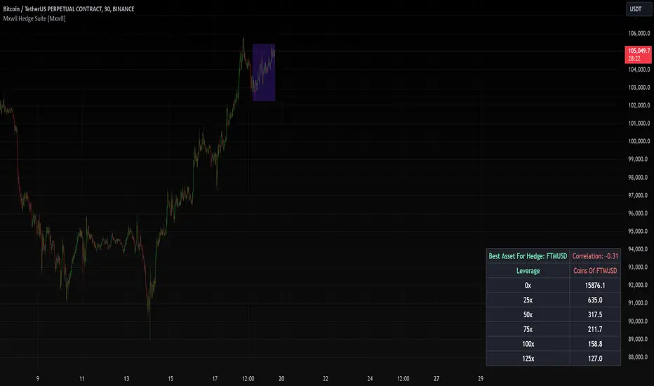
Mxwll Hedge Suite [Mxwll]Hello Traders!
The Mxwll Hedge Suite determines the best asset to hedge against the asset on your chart!
By determining correlation between the asset on your chart and a group of internally listed assets, the Mxwll Hedge Suite determines which asset from the list exhibits the highest negative correlation, and then determines exactly how many coins/shares/contracts of the asset must be bought to achieve a perfect 1:1 hedge!
The image above exemplifies the process!
The purple box on the chart shows the eligible price action used to determine correlation between the asset on my chart (BTCUSDT.P) and the list of cryptocurrencies that can be used as a hedge!
From this price action, the coin determined to have to greatest negative correlation to BTCUSDT.P is FTMUSD.
The image above further outlines the hedge table located in the bottom-right corner of your chart!
The hedge table shows exactly how many coins you’d need to purchase for the hedge asset at various leverages to achieve a perfect 1:1 hedge!
Hedge Suite works on any asset on any timeframe!
And that’s all! A short and sweet script that is hopefully helpful to traders looking to hedge their positions with a negatively correlated asset!
Thank you, Traders!
TTP Pair CipherPair Cipher can run your hedge pair trading strategy.
Pair cipher can use a spread chart (two assets ratio or difference) to manage a hedge position consisting of two assets: one long and one short position.
Event though the spread chart is used to determine the entries and exits each coin price action is used to calculate floating PNL.
It supports different bot platforms. It's backtestable and can run live.
Features:
- Internal and external entry signal
- In-chart realised PNL plot
- Hedge position floating PNL chart
- Individual floating PNL for each long and short ("show coins" toggle)
- Retracement exit strategy: determine at which retracement factor to exit your position while in profit
- PNL RSI exit strategy: determine at which RSI level crossunder you'd like to exit. RSI is applied to the floating PNL
- Static TP/SL levels
- ATR TP/SL levels with individual factors. When ATR is selected the TP or SL acts as a multiplier of ATR instead.
- On-chart debug labels for alerts
- Intra candle alert: signals can trigger intra candle in this mode, but this mode will cause repainting. Example: if the position goes below SL intra candle, the alert will be sent, but later if it goes in profit before closing the candle, the backtest will continue with the position open. The backtest does NOT have access to the intra candle data. Alert intra candle reduces the risk of not applying SL.
Example of setup:
1) Load an empty 1 hour timeframe chart with the spread BYBIT:REQUSDT.P / BYBIT:REEFUSDT.P
2) Select an investment amount
3) Select TP 1.2 and enable ATR
4) Select SL 1.1 and enable ATR
5) Select RSI profits of crossunder 70
6) Don't enable external signal (you can try with TTP PNR)
7) Select BYBIT:REQUSDT.P as symbol 1
8) Select BYBIT:REEFUSDT.P as symbol 2

TTP Alt HedgeAlt hedge is a pine script that allows you to backtest and live hedge trade alt coin pairs.
Once you have selected 20 alt coins and your preferred take profit and a stop loss settings the script will find pairs: one coin that is very overbought and one that is very oversold. It will then long the one in discount and short the premium one.
The script will show you the PNL of the hedge combined position. If together they reach the TP or SL the position will be closed.
Use the "max profit retracement" to target larger TP levels and lock in profits if they retrace more than the chosen ratio. Example: if the TP retraces more than the golden ratio of 0.618 then close the position.
The indicator offers a table of profits with overall PNL and win rate stats.
It can be hooked up to WickHunter bots using alerts and the UUID of the bot.
Debug alerts shows the messages that will be sent for entry/exit deal messages.
Plot PNL shows the cumulative PNL in percentage in the same chart. This function is particularly useful since it shows the performance of the bot.
Each deal in this bot can consist of any pair of coins provided by the user. For example: long ADA + short ETH when ADA is very expensive and ETH is very cheap.
Consider using alt coins that have either strong or vey low correlation, the closer to 1 or -1 in correlation coefficient the better.
Have fun!

Plot the close-spread relationship between two price seriesThis indicator plots the close-spread relationship between two price series by calculating the change across two price series as a spread for each. Each spread is the rate of change in yesterday's closing price and the prior day's closing price. By default, weekend prices are defined to be 0.0 but can be included as user-definable input, if required.
User input:
Symbol for price series 1 - defaults to BITFINEX:BTCUSD
Symbol for price series 2 - defaults to NASDAQ:NDX
Market session time (string) - defaults to 00:00 to 23:59
Timezone - defaults to UTC-4

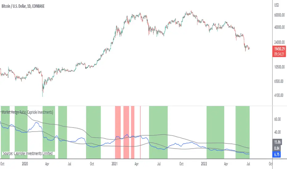
Market Hedge RatioRatio of crypto (total, Bitcoin, or Ethereum market cap) to major stable coins.
A low ratio suggests a lot of people are sitting in cash (sidelined if crypto rallies).
A high ratio suggests possible demand saturation.
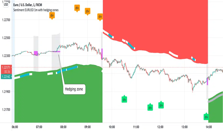
Sentiment EURUSD 1m with hedging zonesThis is a very specialised and optimized script, for 1m EURUSD traders - daytraders, scalpers.
1m trading is very difficult, but it can be also most profitable, if done right.
Why difficult? It is hard to detect market direction - usually when trend indicators reverse, that new trend is already over. One and the same indicator signal sometimes provides one outcome (for example reversal) and sometimes exactly the opposite (continuation). It requires deep understanding on WHEN to use which indicator and when to ignore signals. Set the parameters of your indicators to a very sensitive extent and they will keep changing direction back and forth - always being too late of course :) Set the parameters too losely, and you'll be late with entries 100% of times. Looking for universal trend-showing indicator? There is none...
This script is a result of 2 years of practical following EURUSD 1m market action. Looking at charts with MANUAL TRADER'S eyes. Analyzing all together: price action, indicators, zigzag, divergences, momentum, pivot points, support and resistance. On the one hand traders say only manual trading can be successful and on the other - to stick to one strategy and be automatic when applying to it. So this is it - automatic coding of market signals as if manual trader would do it. Forex is news-driven? Yes, it is. So if market sentiment changes because of some news happening, the script will quickly recognize it and suggest reversal.
Please note I'm not pretending to have a crystal ball. Nobody has. The goal of this script is not to predict where EURUSD market will be, but to correctly notice that is has reversed. Nothing else.
Sometimes the market will move towards reversal, but not cross the line yet - these are so-called HEDGING ZONES. Sometimes they turn out to be reversals and sometimes simply best places for dip entries. Ideally a trader should hedge there, because market could move either way. You might wanna apply apply knowledge of market fundamentals there or look into some micro-indicators. Anyway, it is good to realize where those zones are and this script shows them. In pink.
It is invite-only script. DM me for access.

Yield CurveThis script tracks the U.S. 2Yr/10Yr Spread and uses inversions of the curve to predict recessions. Whenever a red arrow appear on the yield curve, expect a recession to begin within the next 2 years. Use this signal to either exit the market, or hedge current positions. Whenever a green arrow appears on the yield curve, expect a recession to have nearly ended. Use this signal to enter the market, or cut current hedges against a recession. (I may update this script in the future to better incorporate the effective federal funds rate into exit points, but for now I am satisfied with the results).

PC-Indicator - Spar_maDeutsche Version Unterhalb.
English version:
This indicator is supposed to be another tool to recognize when a panic movement has begun and also ended. Of course, there are other indicators that work very well, but this can also help to identify the timeframe.
Description of for using the indicator with the example of the panic sell-off in March:
Before the selloff started, two areas can be identified in which the market is being tested. This is when at the same time, the price intersects with the 21 moving average and the put / call indicator. This indicates that something could be wrong (no guarantee, just an indicator). This happened first (marked with 1) when the virus was discovered: Few who had been informed had any idea what might happen. The second "drop" (marked 2) happened when it was publicly announced that such a virus existed. The third time the panic broke out (marked 3) long after the virus was known. The portfolios should have been hedged here at the latest. Shortly before the yellow marking the virus was reported daily and maximum panic were spread. This was the point at which the hedge could theoretically be ended (if you have the courage to do so). However, I myself waited until the 21st and the indicator were clearly broken.
This indicator could have helped to save a loss in value of the portfolio by at least 17%. I hope this indicator can continue to perform as well.
Please leave a like and subscribe if you are interested in further trading ideas from me.
Name of the indicator: “PC-Indicator - Spar_ma”
That’s my opinion and should be treated like it.
No trade advice!
______________________________________________________________________________________________
Deutsche Version:
Dieser Indikator soll ein weiteres Tool sein um erkennen zu können, wann eine panische Bewegung beendet ist. Natürlich gibt es weitere Indikatoren die sehr gut funktionieren, dieser kann jedoch zusätzlich dabei helfen zu erkennen wann es soweit ist.
Beschreibung des Indikators an Beispiel des Panischen sell-offs im März:
Bereits vor beginn sind zwei Bereiche zu erkennen, an denen der Markt getestet wird. Dabei kreuzen sich gleichzeitig der Kurs mit dem 21-gleitendem Durchschnitt und dem Put-/Call- Indikator. Das lässt darauf zurückführen, dass etwas kommen könnte. Dies geschah zuerst (mit 1 gekennzeichnet) bei der Entdeckung des Virus: Wenige die Informiert wahren, jedoch ahnten was passieren könnte. Der zweite „Drop“ (mit 2 gekennzeichnet) geschah als öffentlich bekannt gegeben wurde, dass ein solches Virus existiert. Beim dritten Mal brach die Panic aus (mit 3 gekennzeichnet), lange nachdem dieser Virus bekannt gewesen war. Spätestens hier sollte das Konto gehedged worden sein. Erst kurz vor der gelben Markierung wurde täglich vom Virus berichtet und maximale Panic verbreitet. Dies war der Zeitpunkt an dem theoretisch der Hedge beendet werden konnte (wenn man den Mut dazu hat). Ich selbst habe allerdings noch gewartet bis der 21ger und auch der Indikator klar durchbrochen wurde.
Dieser Indikator hätte dabei helfen können einen Wertverlust des Kontos um mindestens 17% ersparen zu können. Ich hoffe dieser Indikator kann weiterhin so gut performen.
Bitte lasst ein like da und abonniert mich, falls Ihr Interesse an weiteren trading-ideen von mir habt.
Name des Indikators: “PC-Indicator – Spar_ma”
Dies ist nur meine persönliche Meinung und sollte auch so betrachtet werden.
Dies ist keine Handelsempfehlung.

Cross Pair [NeoButane]Creates candlesticks of a cross pair of any symbol you want. Ideally both pairs would be denominated in the same currency.
The candlesticks are plotted, a close value is available to use for applying indicators on, and a label shows what is being used.
Options to configure are choosing the symbols, displaying the ticker without the exchange name, and removing wicks. If the exchange prefix is 'BATS', 'FRED', or 'TVC', it is automatically removed.

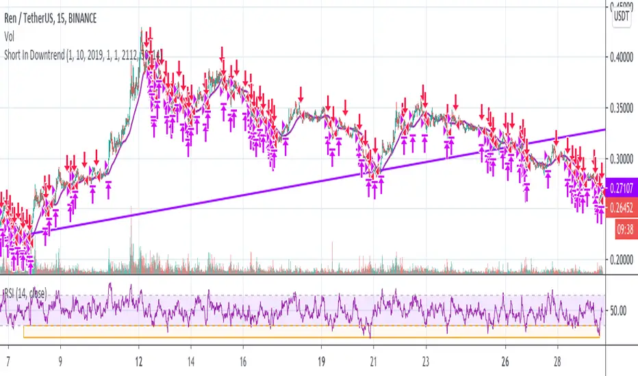
Short In Downtrend Below MA100 (Coinrule)This is a simple strategy to take advantage of downtrends. It's useful to run such a strategy as a hedge in times of market uncertainty.
The Sell Condition - Entry
The sell signal triggers when:
the coin has MA (100) greater than the price in a timeframe of 15 minutes, meaning that the coin is in a short-term downtrend.
the coin has an RSI greater than 30 in a timeframe of 15 minutes, indicating that it didn't reach oversold conditions yet, so there is still room for a further price drop.
On Coinrule, you can launch the strategy on real market conditions, setting up multiple sequential sell orders. The strategy would keep selling while the price stays below the MA(100). In that case, it's advisable to set low amounts for the sell orders. the position will grow gradually while the downtrend intensifies. Set a minimum time interval between the sell orders will also help to have control over the overall position size.
The Buy Condition - Exit
The bot connects to each trade a stop loss and a take profit. The percentages are optimized for short term trades on mid-cap coins. You can adjust the percentages depending on the specific coin you are trading. A ratio of 1:1.5 between the stop loss and the take profit could work as the strategy trades in the same direction of the trend.
Stop loss at 3% from the entry price
Take profit at 2% from the entry price
A slightly larger stop loss allows tolerating more volatility to reduce the case of stops triggering when it shouldn't.
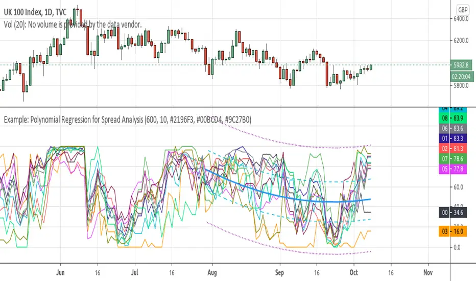
Example: Polynomial Regression for Spread AnalysisExample of applying polynomial regression channel to spreads or hedges between 2 assets.
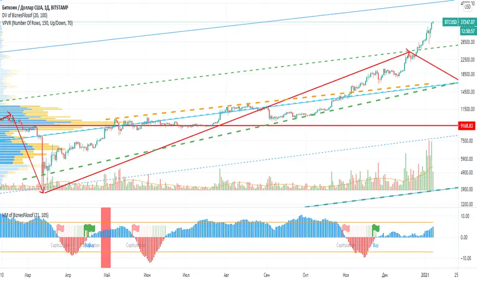
Hashrate Mining of BiznesFilosofIn addition to technical analysis, you also need to pay attention to fundamental analysis. Bitcoin has one of these indicators, it is the network hashrate. And it’s important to know when mining becomes disadvantageous. Those. when network participants turn off the equipment. And there are critical points that depend on the price and number of miners in the network.
When the blue bars of the indicator grow, then you can stand in long. When stools are reduced, then it is time to close positions or hedge risks in the derivatives market.
The vertical line indicates halving.
A red flag indicates a dangerous moment, and a green flag indicates the time of purchase.
The oscillator is based on fundamental indicators and the intersection of moving averages.
===
Кроме теханализа нужно ещё обращать внимание на фундаментальный анализ. У биткоина один из таких показателей, это хэшрейт сети. И важно зать, когда майнинг становится невыгоден. Т.е. когда участники сети отключают оборудование. И есть критические точки, зависящие от цены и количества майнеров в сети.
Когда синие столбики индикатора растут, тогда можно стоять в лонг. Когда столюики уменьшаются, тогда пора закрывать позиции или хеджировать риски на рынке деривативов.
Вертикальной линией обозначен халвинг.
Красный флаг показывает опасный момент, а зелёный флаг указывает на время покупок.
Осцилятор основан на фундаментальных показателях и пересечении скользящих средних.
Commercial Short IndexThis script takes the hedger (commercial short) from the COT report and normalize the chart for configurable time frames (e.g. 26 weeks, 152 weeks and 260 weeks).
Based on the "Commercial Index-Buschi" script by MagicEins.

GRID RELOADED 1.0Script for grid trading on Bitmex XBTUSD 5min
A quick description for the input parameters. I can detail privately the ones that are important:
Points between two same dir trades = how much the price must change before a new DCA can happen
Points between SHORTS = same for short trades
Global Take Profit points = take profit for all open positions expressed in the same units as the price
Global Stop Loss points = same as for profit
Take Profit points decrease per bar = this is how much the target global profit decreases each bar toward zero
Trend up to start a trade long = wait for the DEMA to show a long slope before opening new long positions
Max long position = max n. of long positions
Check trend on trade = wait for a positive/negative bar before long/short
Min Stochastic overbought/sold for trade = wait for the stochastic to be below/above this before long/short
Limit Orders long % below close price = place limit orders % before current price. the order could be left pending.
DEMA 1 Length = periods of DEMA for trends
HA Candles = toggle a pattern match to enter trades

U.S. Stocks & Options CVI to Bitcoin Correlation [NeoButane]Conceptual indicator based on trying to find an inverse correlation between bitcoin and traditional markets due to bitcoin's usefulness as a hedge against economic downturns.
How to use this script: you look at it and see if there is a correlation or not between bitcoin/Ethereum price and either U.S. stock CVi, buy volume, sell volume, calls, puts, or the call/put ratio.

Neo BitMEX Futures Hedge Grid Alerts Premium v1.0This indicator was made to streamline finding the optimal entry to cash and carry/hedge on a futures contract when margin trading.
Explanation of the indicator:
This indicator has built-in alert conditions that you can use to give you email alerts, in-browser sound alerts, or SMS alerts. These alerts are based upon futures prices being in contango or backwardation.
From top to bottom, the grid shows XBTU18, XBTZ18, OkEx's Quarterlies (OKCOIN:BTCUSD3M), and CME's futures.
Red: Futures are trading above your defined range (default 1%) of spot
Maroon: Futures are trading above twice your defined range of spot
Lime: Futures are trading below your defined range (default 1%) of spot
Green: Futures are trading below twice your defined range of spot
What's configurable:
% to trigger
Grid size
Bar color toggle
Label toggle
Spot/index source (Bitfinex's BTCUSD, BitMEX's XBTUSD, and BitMEX's XBT Index are available)
Pricing:
Currently this standalone indicator is 0.007 BTC for lifetime use.
Example of use:
On 4 May 2018, BitMEX's XBTU18 was trading >2% above perpetual swap. The grid alerts signaled that and if one were long on bitcoin spot on any exchange, then it would have been a good idea to hedge a short on XBTU18. Eventually from there the premium gap was closed while bitcoin fell.
Here is the indicator shown with bar coloring and labels.
