RSI with Visual Buy/Sell Setup | Corrective/Impulsive IndicatorRSI with Visual Buy/Sell Setup | 40-60 Support/Resistance | Corrective/Impulsive Indicator v2.15
|| RSI - The Complete Guide PDF ||
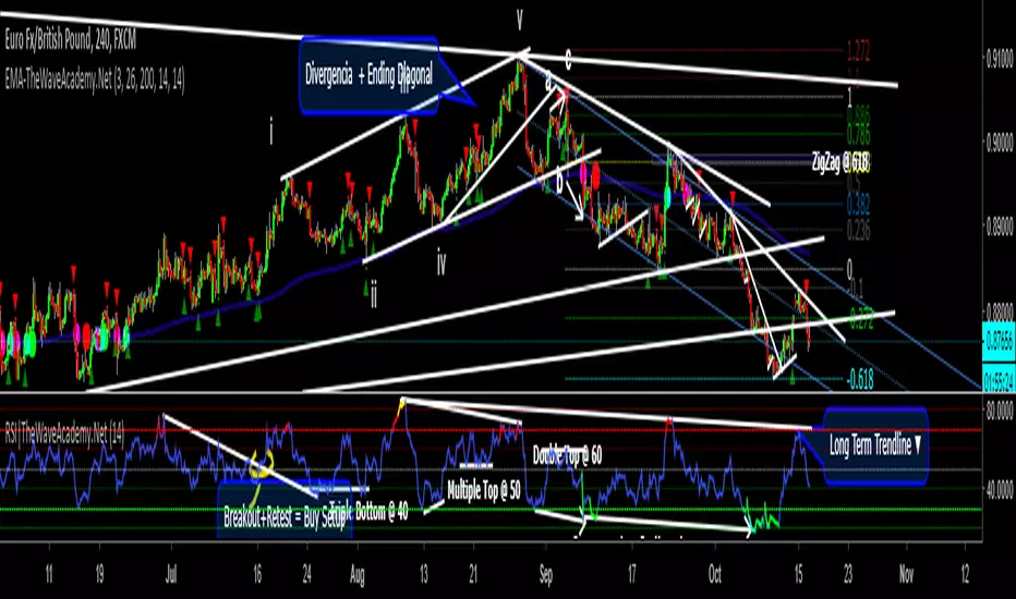
Modified Zones with Colors for easy recognition of Price Action.
Resistance @ downtrend = 60
Support @ uptrend = 40
Over 70 = Strong Bullish Impulse
Under 30 = Strong Bearish Impulse
Uptrend : 40-80
Downtrend: 60-20
--------------------
Higher Highs in price, Lower Highs in RSI = Bearish Divergence
Lower Lows in price, Higher Lows in RSI = Bullish Divergence
--------------------
Trendlines from Higher/Lower Peaks, breakout + retest for buy/sell setups.
###################
There are multiple ways for using RSI, not only divergences, but it confirms the trend, possible bounce for continuation and signals for possible trend reversal.
There's more advanced use of RSI inside the book RSI: The Complete Guide
Go with the force, and follow the trend.
"The Force is more your friend than the trend"
ابحث في النصوص البرمجية عن "股价站上60月线"
Build A Bot Hull TriggerThis is the automated trading system we built during the 60-Minute Build-A-Bot webinar on September 12, 2018. We had a lot of fun, and implemented a TON of indicators LIVE during this webinar! And the best part is that as a group we researched, designed, and built a profitable robot in exactly 60 minutes!
We started by voting on the type of trading system, and this is a trend following system because it got the most votes. Then, the attendees in the webinar sent in their suggestions for indicators and settings during the live webinar (still counting toward the 60 minutes). Once we had the indicators on the chart, and we discussed various settings we could use, we got to work building the robot, and ran the first strategy test...and it was profitable!
This version uses the Hull Moving Average as a trigger for initiating the trade, and everything else is the same for the filters. The other version uses the CCI as a trigger for the trade, and many other indicators as filters.

Indicators: Volume Zone Indicator & Price Zone IndicatorVolume Zone Indicator (VZO) and Price Zone Indicator (PZO) are by Waleed Aly Khalil.
Volume Zone Indicator (VZO)
------------------------------------------------------------
VZO is a leading volume oscillator that evaluates volume in relation to the direction of the net price change on each bar.
A value of 40 or above shows bullish accumulation. Low values (< 40) are bearish. Near zero or between +/- 20, the market is either in consolidation or near a break out. When VZO is near +/- 60, an end to the bull/bear run should be expected soon. If that run has been opposite to the long term price trend direction, then a reversal often will occur.
Traditional way of looking at this also works:
* +/- 40 levels are overbought / oversold
* +/- 60 levels are extreme overbought / oversold
More info:
drive.google.com
Price Zone Indicator (PZO)
------------------------------------------------------------
PZO is interpreted the same way as VZO (same formula with "close" substituted for "volume").
Chart Markings
------------------------------------------------------------
In the chart above,
* The red circles indicate a run-end (or reversal) zones (VZO +/- 60).
* Blue rectangle shows the consolidation zone (VZO betwen +/- 20)
I have been trying out VZO only for a week now, but I think this has lot of potential. Give it a try, let me know what you think.

Echo Chamber [theUltimator5]The Echo Chamber - When history repeats, maybe you should listen.
Ever had that eerie feeling you've seen this exact price action before? The Echo Chamber doesn't just give you déjà vu—it mathematically proves it, scales it, and projects what happened next.
📖 WHAT IT DOES
The Echo Chamber is an advanced pattern recognition tool that scans your chart's history to find segments that closely match your current price action. But here's where it gets interesting: it doesn't just find similar patterns - It expands and contracts the time window to create a uniquely scaled fractal. Patterns don't always follow the same timeframe, but they do follow similar patterns.
Using a custom correlation analysis algorithm combined with flexible time-scaling, this indicator:
Finds historical price segments that mirror your current market structure
Scales and overlays them perfectly onto your current chart
Projects forward what happened AFTER that historical match
Gives you a visual "echo" from the past with a glimpse into potential futures
══════════════════════════════
HOW TO USE IT
This indicator starts off in manual mode, which means that YOU, the user, can select the point in time that you want to project from. Simply click on a point in time to set the starting value.
Once you select your point in time, the indicator will automatically plot the chosen historical chart pattern and correlation over the current chart and project the price forwards based on how the chart looked in the past. If you want to change the point in time, you can update it from the settings, or drag the point on the chart over to a new position.
You can manually select any point in time, and the chart will quickly update with the new pattern. A correlation will be shown in a table alongside the date/timestamp of the selected point in time.
You can switch to auto mode, which will automatically search out the best-fit pattern over a defined lookback range and plot the past/future projection for you without having to manually select a point in time at all. It simply finds the best fit for you.
You can change the scale factor by adjusting multiplication and division variables to find time-scaled fractal patterns.
══════════════════════════════
🎯 KEY FEATURES
Two Operating Modes:
🔧 MANUAL MODE - Select any historical point and see how it correlates with current price action in real-time. Perfect for:
• Analyzing specific past events (crashes, rallies, consolidations)
• Testing historical patterns against current conditions
• Educational analysis of market structure repetition
🤖 AUTO MODE - It automatically scans through your lookback period to find the single best-correlated historical match. Ideal for:
• Quick pattern discovery
• Systematic trading approach
• Unbiased pattern recognition
Time Warp Technology:
The time warp feature expands and compresses the correlation window to provide a custom fractal so you can analyze windows of time that don't necessarily match the current chart.
💡 *Example: Multiplier=3, Divisor=2 gives you a 1.5x time stretch—perfect for finding patterns that played out 50% slower than current price action.*
Drawing Modes:
Scale Only : Pure vertical scaling—matches price range while maintaining temporal alignment at bar 0
Rotate & Scale : Advanced geometric transformation that anchors both the start AND end points, creating a rotated fit that matches your current segment's slope and range
Visual Components:
🟠 Orange Overlay : The historical match, perfectly scaled to your current price action
🟣 Purple Projection : What happened NEXT after that historical pattern (dotted line into the future)
📦 Highlight Boxes : Shows you exactly where in history these patterns came from
📊 Live Correlation Table : Real-time correlation coefficient with color-coded strength indicator
══════════════════════════════
⚙️ PARAMETERS EXPLAINED
Correlation Window Length (20) : How many bars to match. Smaller = more precise matches but noisier. Larger = broader patterns but fewer matches.
Note: if this value is too high in auto mode, the script may time out from computational overload.
Multiplication Factor : Historical time multiplier. 2 = sample every 2nd bar from history. Higher values find slower historical patterns.
Division Factor : Historical time divisor applied after multiplication. Final sample rate = (Length × Factor) ÷ Divisor, rounded down.
Lookback Range : How far back to search for patterns. More history = better chance of finding matches but slower performance.
Note: if this value is too high in auto mode, the script may time out from computational overload.
Future Projection Length : How many bars forward to project from the historical match. Your crystal ball's focal length.
══════════════════════════════
💼 TRADING APPLICATIONS
Trend Continuation/Reversal :
If the purple projection continues the current trend, that's your historical confirmation. If it reverses, you've found a potential turning point that's happened before under similar conditions.
Support/Resistance Validation :
Does the projection respect your S/R levels? History suggests those levels matter. Does it break through? You've found historical precedent for a breakout.
Time-Based Exits :
The projection shows not just WHERE price might go, but WHEN. Use it to anticipate timing of moves.
Multi-Timeframe Analysis :
Use time compression to overlay higher timeframe patterns onto lower timeframes. See daily patterns on hourly charts, weekly on daily, etc.
Pattern Education :
In Manual Mode, study how specific historical events correlate with current conditions. Build your pattern recognition library.
══════════════════════════════
📊 CORRELATION TABLE
The table shows your correlation coefficient as a percentage:
80-100%: Extremely strong correlation—history is practically repeating
60-80%: Strong correlation—significant similarity
40-60%: Moderate correlation—some structural similarity
20-40%: Weak correlation—limited similarity
0-20%: Very weak correlation—essentially random match
-20-40%: Weak inverse correlation
-40-60%: Moderate inverse correlation
-60-80%: Strong inverse correlation
-80-100%: Extremely strong inverse correlation—history is practically inverting
**Important**: The correlation measures SHAPE similarity, not price level. An 85% correlation means the price movements follow a very similar pattern, regardless of whether prices are higher or lower.
══════════════════════════════
⚠️ IMPORTANT DISCLAIMERS
- Past performance does NOT guarantee future results (but it sure is interesting to study)
- High correlation doesn't mean causation—markets are complex adaptive systems
- Use this as ONE tool in your analytical toolkit, not a standalone trading system
- The projection is what HAPPENED after a similar pattern in the past, not a prediction
- Always use proper risk management regardless of what the Echo Chamber suggests
══════════════════════════════
🎓 PRO TIPS
1. Start with Auto Mode to find high-correlation matches, then switch to Manual Mode to study why that period was similar
2. Experiment with time warping on different timeframes—a 2x factor on a daily chart lets you see weekly patterns
3. Watch for correlation decay —if correlation drops sharply after the match, current conditions are diverging from history
4. Combine with volume —check if volume patterns also match
5. Use "Rotate & Scale" mode when the current trend angle differs from the historical match
6. Increase lookback range to 500-1000+ on daily/weekly charts for finding rare historical parallels
══════════════════════════════
🔧 TECHNICAL NOTES
- Uses Pearson correlation coefficient for pattern matching
- Implements range-based scaling to normalize different price levels
- Rotation mode uses linear interpolation for geometric transformation
- All calculations are performed on close prices
- Boxes highlight actual historical bar ranges (high/low)
- Maximum of 500 lines and 500 boxes for performance optimization

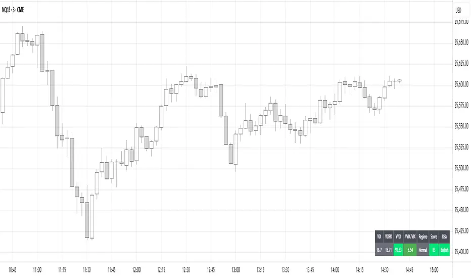
Volatility Regime NavigatorA guide to understanding VIX, VVIX, VIX9D, VVIX/VIX, and the Composite Risk Score
1. Purpose of the Indicator
This dashboard summarizes short-term market volatility conditions using four core volatility metrics.
It produces:
• Individual readings
• A combined Regime classification
• A Composite Risk Score (0–100)
• A simplified Risk Bucket (Bullish → Stress)
Use this to evaluate market fragility, drift potential, tail-risk, and overall risk-on/off conditions.
This is especially useful for intraday ES/NQ trading, expected-move context, and understanding when breakouts or fades have edge.
2. The Four Core Volatility Inputs
(1) VIX — Baseline Equity Volatility
• < 16: Complacent (easy drift-up, but watch for fragility)
• 16–22: Healthy, normal volatility → ideal trading conditions
• > 22: Stress rising
• > 26: Tail-risk / risk-off environment
(2) VIX9D — Short-Term Event Vol
Measures 9-day implied volatility. Reacts to immediate news/events.
• < 14: Strongly bullish (drift regime)
• 14–17: Bullish to neutral
• 17–20: Event risk building
• > 20: Short-term stress / caution
(3) VVIX — Volatility of VIX (fragility index)
Tracks volatility of volatility.
• < 100: “Bullish, Bullish” — very low fragility
• 100–120: Normal
• 120–140: Fragile
• > 140: Stress, hedging pressure
(4) VVIX/VIX Ratio — Microstructure Risk-On/Risk-Off
One of the most sensitive indicators of market confidence.
• 5.0–6.5: Strongest “normal/bullish” zone
• < 5.0: Bottom-stalking / fear regime
• > 6.5: Complacency → vulnerable to reversals
• > 7.5: Fragile / top-risk
3. Composite Risk Score (0–100)
The dashboard converts all four inputs into a single score.
Score Interpretation
• 80–100 → Bullish - Drift regime. Shallow pullbacks. Upside favored.
• 60–79 → Normal - Healthy tape. Balanced two-way trading.
• 40–59 → Fragile - Choppy, failed breakouts, thinner liquidity.
• 20–39 → Risk-Off - Downside tails active. Favor fades and defensive behavior.
• < 20 → Stress - Crisis or event-driven tape. Avoid longs.
Score updates every bar.
4. Regime Label
Independent of the composite score, the script provides a Regime classification based on combinations of VIX + VVIX/VIX:
• Bullish+ → Buying is easy, tape lifts passively
• Normal → Cleanest and most tradable conditions
• Complacent → Top-risk; be careful chasing upside
• Mixed → Signals conflict; chop potential
• Bottom Stalk → High VIX, low VVIX/VIX (capitulation signatures)
A trailing “+” or “*” indicates additional bullish or caution overlays from VIX9D/VVIX.
5. How to Use the Dashboard in Trading
When Bullish (Score ≥ 80):
• Expect drift-up behavior
• Downside limited unless catalyst hits
• Structure favors breakouts and trend continuation
• Mean reversion trades have lower expectancy
When Normal (Score 60–79):
• The “playbook regime”
• Breakouts and mean reversion both valid
• Best overall trading environment
When Fragile (Score 40–59):
• Expect chop
• Breakouts fail
• Take quicker profits
• Avoid overleveraged directional bets
When Risk-Off (20–39):
• Favor fades of strength
• Downside tails activate
• Trend-following short setups gain edge
• Respect volatility bands
When Stress (<20):
• Avoid long exposure
• Do not chase dips
• Expect violent, news-sensitive behavior
• Position sizing becomes critical
6. Quick Summary
• VIX = weather
• VIX9D = short-term storm radar
• VVIX = foundation stability
• VVIX/VIX = confidence vs fragility
• Composite Score = overall regime health
• Risk Bucket = simple “what do I do?” label
This dashboard gives traders a high-confidence, low-noise view of equity volatility conditions in real time.
Dual TF Bearish Divergence (Working)//@version=6
indicator("Dual TF Bearish Divergence (Working)", overlay=true)
// ----------------- SIMPLE BEARISH DIVERGENCE FUNCTION -------------------
bearDiv(src, rsiLen, lookbackMin, lookbackMax) =>
r = ta.rsi(src, rsiLen)
ph = ta.pivothigh(src, lookbackMin, lookbackMin)
ph_rsi = ta.pivothigh(r, lookbackMin, lookbackMin)
ph2 = ph
ph2_rsi = ph_rsi
priceHH = not na(ph) and not na(ph2) and ph > ph2
rsiLH = not na(ph_rsi) and not na(ph2_rsi) and ph_rsi < ph2_rsi
barsOk = lookbackMin >= lookbackMin and lookbackMin <= lookbackMax
priceHH and rsiLH and barsOk
// ----------------- TF CALLS -------------------
b60 = request.security(syminfo.tickerid, "60", bearDiv(close, 14, 10, 15))
b240 = request.security(syminfo.tickerid, "240", bearDiv(close, 14, 10, 15))
dual = b60 and b240
// ----------------- PLOT -------------------
plotshape(dual, title="Dual Bear Div", style=shape.labeldown,
color=color.red, size=size.small, text="🔻BearDiv")
// ----------------- ALERT -------------------
alertcondition(dual, "Dual Bearish Div 60+240",
"Bearish Divergence on both 60m & 240m")

Reversal_Detector//@version=6
indicator("상승 반전 탐지기 (Reversal Detector)", overlay=true)
// ==========================================
// 1. 설정 (Inputs)
// ==========================================
rsiLen = input.int(14, title="RSI 길이")
lbR = input.int(5, title="다이버전스 확인 범위 (오른쪽)")
lbL = input.int(5, title="다이버전스 확인 범위 (왼쪽)")
rangeUpper = input.int(60, title="RSI 과매수 기준")
rangeLower = input.int(30, title="RSI 과매도 기준")
// ==========================================
// 2. RSI 상승 다이버전스 계산 (핵심 로직)
// ==========================================
osc = ta.rsi(close, rsiLen)
// 피벗 로우(Pivot Low) 찾기: 주가의 저점
plFound = na(ta.pivotlow(osc, lbL, lbR)) ? false : true
// 다이버전스 조건 확인
// 1) 현재 RSI 저점이 이전 RSI 저점보다 높아야 함 (상승)
// 2) 현재 주가 저점이 이전 주가 저점보다 낮아야 함 (하락)
showBull = false
if plFound
// 이전 피벗 지점 찾기
oscLow = osc
priceLow = low
// 과거 데이터를 탐색하여 직전 저점과 비교
for i = 1 to 60
if not na(ta.pivotlow(osc, lbL, lbR) ) // 이전에 저점이 있었다면
prevOscLow = osc
prevPriceLow = low
// 다이버전스 조건: 가격은 더 떨어졌는데(Lower Low), RSI는 올랐을 때(Higher Low)
if priceLow < prevPriceLow and oscLow > prevOscLow and oscLow < rangeLower
showBull := true
break // 하나 찾으면 루프 종료
// ==========================================
// 3. 보조 조건 (MACD 골든크로스 & 이평선)
// ==========================================
= ta.macd(close, 12, 26, 9)
macdCross = ta.crossover(macdLine, signalLine) // MACD 골든크로스
ma5 = ta.sma(close, 5)
ma20 = ta.sma(close, 20)
maCross = ta.crossover(ma5, ma20) // 5일선이 20일선 돌파
// ==========================================
// 4. 시각화 (Plotting)
// ==========================================
// 1) 상승 다이버전스 발생 시 (강력한 바닥 신호)
plotshape(showBull,
title="상승 다이버전스",
style=shape.labelup,
location=location.belowbar,
color=color.red,
textcolor=color.white,
text="Bull Div\n(바닥신호)",
size=size.small,
offset=-lbR) // 과거 시점에 표시
// 2) MACD 골든크로스 (추세 확인용)
plotshape(macdCross and macdLine < 0, // 0선 아래에서 골든크로스 날 때만
title="MACD 골든크로스",
style=shape.triangleup,
location=location.belowbar,
color=color.yellow,
size=size.tiny,
text="MACD")
// 3) 이동평균선
plot(ma5, color=color.blue, title="5일선")
plot(ma20, color=color.orange, title="20일선")
// 알림 설정
alertcondition(showBull, title="상승 다이버전스 포착", message="상승 다이버전스 발생! 추세 반전 가능성")

Trend Trader//@version=6
indicator("Trend Trader", shorttitle="Trend Trader", overlay=true)
// User-defined input for moving averages
shortMA = input.int(10, minval=1, title="Short MA Period")
longMA = input.int(100, minval=1, title="Long MA Period")
// User-defined input for the instrument selection
instrument = input.string("US30", title="Select Instrument", options= )
// Set target values based on selected instrument
target_1 = instrument == "US30" ? 50 :
instrument == "NDX100" ? 25 :
instrument == "GER40" ? 25 :
instrument == "GOLD" ? 5 : 5 // default value
target_2 = instrument == "US30" ? 100 :
instrument == "NDX100" ? 50 :
instrument == "GER40" ? 50 :
instrument == "GOLD" ? 10 : 10 // default value
// User-defined input for the start and end times with default values
startTimeInput = input.int(12, title="Start Time for Session (UTC, in hours)", minval=0, maxval=23)
endTimeInput = input.int(17, title="End Time Session (UTC, in hours)", minval=0, maxval=23)
// Convert the input hours to minutes from midnight
startTime = startTimeInput * 60
endTime = endTimeInput * 60
// Function to convert the current exchange time to UTC time in minutes
toUTCTime(exchangeTime) =>
exchangeTimeInMinutes = exchangeTime / 60000
// Adjust for UTC time
utcTime = exchangeTimeInMinutes % 1440
utcTime
// Get the current time in UTC in minutes from midnight
utcTime = toUTCTime(time)
// Check if the current UTC time is within the allowed timeframe
isAllowedTime = (utcTime >= startTime and utcTime < endTime)
// Calculating moving averages
shortMAValue = ta.sma(close, shortMA)
longMAValue = ta.sma(close, longMA)
// Plotting the MAs
plot(shortMAValue, title="Short MA", color=color.blue)
plot(longMAValue, title="Long MA", color=color.red)
// MACD calculation for 15-minute chart
= request.security(syminfo.tickerid, "15", ta.macd(close, 12, 26, 9))
macdColor = macdLine > signalLine ? color.new(color.green, 70) : color.new(color.red, 70)
// Apply MACD color only during the allowed time range
bgcolor(isAllowedTime ? macdColor : na)
// Flags to track if a buy or sell signal has been triggered
var bool buyOnce = false
var bool sellOnce = false
// Tracking buy and sell entry prices
var float buyEntryPrice_1 = na
var float buyEntryPrice_2 = na
var float sellEntryPrice_1 = na
var float sellEntryPrice_2 = na
if not isAllowedTime
buyOnce :=false
sellOnce :=false
// Logic for Buy and Sell signals
buySignal = ta.crossover(shortMAValue, longMAValue) and isAllowedTime and macdLine > signalLine and not buyOnce
sellSignal = ta.crossunder(shortMAValue, longMAValue) and isAllowedTime and macdLine <= signalLine and not sellOnce
// Update last buy and sell signal values
if (buySignal)
buyEntryPrice_1 := close
buyEntryPrice_2 := close
buyOnce := true
if (sellSignal)
sellEntryPrice_1 := close
sellEntryPrice_2 := close
sellOnce := true
// Apply background color for entry candles
barcolor(buySignal or sellSignal ? color.yellow : na)
/// Creating buy and sell labels
if (buySignal)
label.new(bar_index, low, text="BUY", style=label.style_label_up, color=color.green, textcolor=color.white, yloc=yloc.belowbar)
if (sellSignal)
label.new(bar_index, high, text="SELL", style=label.style_label_down, color=color.red, textcolor=color.white, yloc=yloc.abovebar)
// Creating labels for 100-point movement
if (not na(buyEntryPrice_1) and close >= buyEntryPrice_1 + target_1)
label.new(bar_index, high, text=str.tostring(target_1), style=label.style_label_down, color=color.green, textcolor=color.white, yloc=yloc.abovebar)
buyEntryPrice_1 := na // Reset after label is created
if (not na(buyEntryPrice_2) and close >= buyEntryPrice_2 + target_2)
label.new(bar_index, high, text=str.tostring(target_2), style=label.style_label_down, color=color.green, textcolor=color.white, yloc=yloc.abovebar)
buyEntryPrice_2 := na // Reset after label is created
if (not na(sellEntryPrice_1) and close <= sellEntryPrice_1 - target_1)
label.new(bar_index, low, text=str.tostring(target_1), style=label.style_label_up, color=color.red, textcolor=color.white, yloc=yloc.belowbar)
sellEntryPrice_1 := na // Reset after label is created
if (not na(sellEntryPrice_2) and close <= sellEntryPrice_2 - target_2)
label.new(bar_index, low, text=str.tostring(target_2), style=label.style_label_up, color=color.red, textcolor=color.white, yloc=yloc.belowbar)
sellEntryPrice_2 := na // Reset after label is created

Smart MACD Divergence ScannerOriginal Base Indicator: "CM_MacD_Ult_MTF" by ChrisMoody
This indicator builds upon ChrisMoody's excellent multi-timeframe MACD foundation and transforms it into a professional divergence scanner with advanced quality assessment and filtering capabilities. The original MACD visualization and MTF functionality have been preserved while adding completely new divergence detection, scoring, and filtering systems.
🎯 What Makes This Indicator Unique:
Smart MACD Divergence Scanner is a professional tool for detecting MACD-based divergences with an advanced filtering system and signal quality assessment. Unlike standard divergence indicators, this version includes innovative features:
Adaptive Quality Scoring System — each signal receives a score from 0 to 100 based on multiple factors
Volatility Filter — automatic signal suppression during low market volatility periods
Multi-Timeframe Confirmation — divergence verification on higher timeframe for increased reliability
Divergence Strength Analysis — calculation of percentage difference between price and indicator movement
Information Dashboard — detailed real-time signal statistics
Cooldown System — prevention of multiple consecutive signals
💡 How It Works:
The indicator uses the classic divergence concept — the divergence between price movement and the MACD oscillator. However, instead of simple pivot detection, the algorithm:
Scans the market for local extremes (pivots) on price and MACD histogram
Searches for divergences — when price updates low/high while MACD shows opposite movement
Assesses quality — analyzes divergence strength, volatility, higher timeframe confirmation
Filters noise — eliminates weak signals through threshold system and cooldown
Generates signal — only when all quality criteria are met
🔧 Key Parameters:
MACD Settings: Fast Length (12), Slow Length (26), Signal Length (9)
Divergence Detection: Pivot Lookback (5), Max Lookback Range (60), Min Divergence Strength (15%)
Quality Filters: Min Quality Score (60), Volatility Filter, MTF Confirmation, Signal Cooldown (5)
📊 How to Use:
Add indicator to chart — it will automatically start scanning
Configure filters — start with default settings, then adapt to your trading style
Watch for signals: 🟢 Green "BUY" label = bullish divergence, 🔴 Red "SELL" label = bearish divergence
Check quality score on labels (Q: XX)
Use information panel to monitor statistics and current market conditions
⚙️ Settings Guide:
For swing trading (4H-Daily): Increase Pivot Lookback to 7-10, set Min Quality Score to 70+
For day trading (15m-1H): Keep default settings, enable all filters
For scalping (1m-5m): Decrease Min Quality Score to 50, disable MTF Confirmation
For volatile markets (crypto): Increase Min Divergence Strength to 20-25%, enable Volatility Filter
⚠️ Important Notes:
Divergences are probabilistic signals, not guaranteed reversals
Use additional confirmation (support/resistance levels, volume, price action)
Adjust parameters for specific asset and timeframe
Signals appear with Pivot Lookback bars delay (retrospective confirmation)
On volatile markets, increase Min Quality Score to reduce false signals

GRA v5 SNIPER# GRA v5 SNIPER - Documentation & Cheatsheet
## 🎯 Get Rich Aggressively v5 - SNIPER Edition
**Precision Futures Scalping | NQ • ES • YM • GC • BTC**
> **Philosophy:** *Quality over quantity. One sniper shot beats ten spray-and-pray attempts.*
---
## ⚡ QUICK CHEATSHEET
```
┌─────────────────────────────────────────────────────────────────────────────┐
│ GRA v5 SNIPER - QUICK REFERENCE │
├─────────────────────────────────────────────────────────────────────────────┤
│ │
│ 🎯 SIGNAL REQUIREMENTS (ALL MUST BE TRUE): │
│ ═══════════════════════════════════════════ │
│ ✓ Tier → B minimum (20+ pts NQ) │
│ ✓ Volume → 1.5x+ average │
│ ✓ Delta → 60%+ dominance (buyers OR sellers) │
│ ✓ Body → 70%+ of candle range │
│ ✓ Range → 1.3x+ average candle size │
│ ✓ Wicks → Small opposite wick (<50% of body) │
│ ✓ CVD → Trending with signal direction │
│ ✓ Session → London (3-5am ET) OR NY (9:30-11:30am ET) │
│ │
├─────────────────────────────────────────────────────────────────────────────┤
│ │
│ 📊 TIER ACTIONS: │
│ ════════════════ │
│ S-TIER (100+ pts) → 🥇 HOLD position, ride the wave │
│ A-TIER (50-99 pts) → 🥈 SWING for 2-3 minutes │
│ B-TIER (20-49 pts) → 🥉 SCALP quick, 30-60 seconds │
│ │
├─────────────────────────────────────────────────────────────────────────────┤
│ │
│ 🚨 ENTRY CHECKLIST: │
│ ═══════════════════ │
│ □ Signal appears (S🎯, A🎯, or B🎯) │
│ □ Table shows: Vol GREEN, Delta colored, Body GREEN │
│ □ CVD arrow matches direction (▲ for long, ▼ for short) │
│ □ Session active (LDN! or NY! in yellow) │
│ □ Enter at close of signal candle │
│ │
├─────────────────────────────────────────────────────────────────────────────┤
│ │
│ ⛔ DO NOT TRADE WHEN: │
│ ════════════════════ │
│ ✗ Session shows "---" (outside key hours) │
│ ✗ Vol shows RED (below 1.5x) │
│ ✗ Body shows RED (weak candle structure) │
│ ✗ Delta below 60% (no clear dominance) │
│ ✗ Multiple conflicting signals │
│ │
├─────────────────────────────────────────────────────────────────────────────┤
│ │
│ 📈 INSTRUMENT SETTINGS: │
│ ════════════════════════ │
│ NQ/ES (1-3 min): S=100, A=50, B=20 pts │
│ YM (1-5 min): S=100, A=50, B=25 pts │
│ GC (5-15 min): S=15, A=8, B=4 pts │
│ BTC (1-15 min): S=500, A=250, B=100 pts │
│ │
└─────────────────────────────────────────────────────────────────────────────┘
```
---
## 📋 DETAILED DOCUMENTATION
### What Makes SNIPER Different?
The SNIPER edition eliminates 80%+ of signals compared to standard GRA. Every signal that passes through has been validated by **8 independent filters**:
| Filter | Standard GRA | SNIPER GRA | Why It Matters |
|--------|-------------|------------|----------------|
| Volume | 1.3x avg | **1.5x avg** | Institutional participation |
| Delta | 55% | **60%** | Clear buyer/seller control |
| Body Ratio | None | **70%+** | No dojis or spinners |
| Range | None | **1.3x avg** | Significant price movement |
| Wicks | None | **<50% body** | Conviction in direction |
| CVD | None | **Required** | Trend confirmation |
| B-Tier Min | 10 pts | **20 pts** | Filter noise |
| Session | Optional | **Required** | Institutional hours |
---
### Signal Anatomy
When you see a signal like `A🎯`, here's what passed validation:
```
Signal: A🎯 LONG at 21,450.00
Validation Breakdown:
├── Points: 67.5 pts ✓ (A-Tier = 50-99)
├── Volume: 2.1x avg ✓ (≥1.5x required)
├── Delta: 68% Buyers ✓ (≥60% required)
├── Body: 78% of range ✓ (≥70% required)
├── Range: 1.6x avg ✓ (≥1.3x required)
├── Wick: Upper 15% ✓ (<50% of body)
├── CVD: ▲ Rising ✓ (Matches LONG)
└── Session: NY! ✓ (Active session)
RESULT: VALID SNIPER SIGNAL
```
---
### Table Legend
| Field | Reading | Color Meaning |
|-------|---------|---------------|
| **Pts** | Point movement | Gold/Green/Yellow = Tiered |
| **Tier** | S/A/B/X | Gold/Green/Yellow/White |
| **Vol** | Volume ratio | 🟢 ≥1.5x, 🔴 <1.5x |
| **Delta** | Buy/Sell % | 🟢 Buy dom, 🔴 Sell dom, ⚪ Neutral |
| **Body** | Body % of range | 🟢 ≥70%, 🔴 <70% |
| **CVD** | Cumulative delta | ▲ Bullish trend, ▼ Bearish trend |
| **Sess** | Session status | 🟡 Active, ⚫ Inactive |
---
### Trading Rules
#### Entry Rules
1. **Wait for signal** - Don't anticipate
2. **Verify table** - All conditions GREEN
3. **Enter at candle close** - Not during formation
4. **Position size by tier:**
- S-Tier: Full size
- A-Tier: 75% size
- B-Tier: 50% size
#### Exit Rules
| Tier | Target | Max Hold Time |
|------|--------|---------------|
| S | Let it run | 5-10 minutes |
| A | 1:1.5 R:R | 2-3 minutes |
| B | 1:1 R:R | 30-60 seconds |
#### Stop Loss
- Place at **opposite end of signal candle**
- For S-Tier: Allow 50% retracement
- For B-Tier: Tight stop, quick exit
---
### Session Priority
```
LONDON OPEN (3:00-5:00 AM ET)
════════════════════════════
• Best for: GC, European indices
• Characteristics: Stop hunts, reversals
• Look for: Sweeps of Asian session levels
NY OPEN (9:30-11:30 AM ET)
════════════════════════════
• Best for: NQ, ES, YM
• Characteristics: High volume, trends
• Look for: Continuation after 10 AM
```
---
### Common Mistakes to Avoid
| Mistake | Why It's Bad | Solution |
|---------|-------------|----------|
| Trading outside sessions | Low volume = fake moves | Wait for LDN! or NY! |
| Ignoring weak body | Dojis reverse | Body must be 70%+ |
| Fighting CVD | Swimming upstream | CVD must confirm |
| Oversizing B-Tier | Small moves = small size | 50% max on B |
| Chasing missed signals | FOMO loses money | Wait for next setup |
---
### Alert Setup
Configure these alerts in TradingView:
| Alert | Priority | Action |
|-------|----------|--------|
| 🎯 S-TIER LONG/SHORT | 🔴 High | Drop everything, check chart |
| 🎯 A-TIER LONG/SHORT | 🟠 Medium | Evaluate within 30 seconds |
| 🎯 B-TIER LONG/SHORT | 🟢 Low | Quick glance if available |
| LONDON/NY OPEN | 🔵 Info | Prepare for action |
---
### Pine Script v6 Notes
This indicator uses Pine Script v6 features:
- `request.security_lower_tf()` for intrabar delta
- Type inference for cleaner code
- Array operations for CVD calculation
**Minimum TradingView Plan:** Pro (for intrabar data)
---
## 🏆 Golden Rule
> **"If you have to convince yourself it's a good signal, it's not a good signal."**
The SNIPER edition is designed so that when a signal appears, there's nothing to think about. If all conditions are met, you trade. If any condition fails, you wait.
**Leave every trade with money. That's the goal.**
---
*© Alexandro Disla - Get Rich Aggressively v5 SNIPER*
*Pine Script v6 | TradingView*

Sideways & Breakout Detector + Forecast//@version=6
indicator("Sideways & Breakout Detector + Forecast", overlay=true, max_labels_count=500)
// Inputs
lengthATR = input.int(20, "ATR Länge")
lengthMA = input.int(50, "Trend MA Länge")
sqFactor = input.float(1.2, "Seitwärtsfaktor")
brkFactor = input.float(1.5, "Breakoutfaktor")
// ATR / Volatilität
atr = ta.atr(lengthATR)
atrSMA = ta.sma(atr, lengthATR)
// Basislinie / Trend
basis = ta.sma(close, lengthATR)
trendMA = ta.sma(close, lengthMA)
// Seitwärtsbedingung
isSideways = atr < atrSMA * sqFactor
// Breakouts
upperBreak = close > basis + atr * brkFactor
lowerBreak = close < basis - atr * brkFactor
// Vorhergesagter Ausbruch (Forecast)
// Wenn Seitwärtsphase + Kurs nahe obere oder untere Kanalgrenze
forecastBull = isSideways and (close > basis + 0.5 * atr)
forecastBear = isSideways and (close < basis - 0.5 * atr)
// Farben
barcolor(isSideways ? color.new(color.yellow, 40) : na)
barcolor(upperBreak ? color.green : na)
barcolor(lowerBreak ? color.red : na)
// Breakout-Bänder
plot(basis + atr * brkFactor, "Bull Break Zone", color=color.new(color.green, 60))
plot(basis - atr * brkFactor, "Bear Break Zone", color=color.new(color.red, 60))
// Labels (klein)
if isSideways
label.new(bar_index, close, "Seitwärts", color=color.yellow, style=label.style_label_center, size=size.tiny)
if upperBreak
label.new(bar_index, high, "Bull Breakout", color=color.green, style=label.style_label_up, size=size.tiny)
if lowerBreak
label.new(bar_index, low, "Bear Breakout", color=color.red, style=label.style_label_down, size=size.tiny)
// Vorhergesagte Ausbrüche markieren
plotshape(forecastBull, title="Forecast Bull", location=location.abovebar, color=color.new(color.green, 0), style=shape.triangleup, size=size.tiny)
plotshape(forecastBear, title="Forecast Bear", location=location.belowbar, color=color.new(color.red, 0), style=shape.triangledown, size=size.tiny)
// Alerts
alertcondition(isSideways, "Seitwärtsphase", "Der Markt läuft seitwärts.")
alertcondition(upperBreak, "Bull Breakout", "Ausbruch nach oben!")
alertcondition(lowerBreak, "Bear Breakout", "Ausbruch nach unten!")
alertcondition(forecastBull, "Forecast Bull", "Voraussichtlicher Bull-Ausbruch!")
alertcondition(forecastBear, "Forecast Bear", "Voraussichtlicher Bear-Ausbruch!")

Stratégie SMC V18.2 (BTC/EUR FINAL R3 - Tendance)This strategy is an automated implementation of Smart Money Concepts (SMC), designed to operate on the Bitcoin/Euro (BTC/EUR) chart using the 15-minute Timeframe (M15).It focuses on identifying high-probability zones (Order Blocks) after a confirmed Break of Structure (BOS) and a Liquidity Sweep, utilizing an H1/EMA 200 trend filter to only execute trades in the direction of the dominant market flow.Risk management is strict: every trade uses a fixed Risk-to-Reward Ratio (R:R) of 1:3.🧱 Core Logic Components
1. Trend Filter (H1/EMA 200)Objective: To avoid counter-trend entries, which has allowed the success rate to increase to nearly $65\%$ in backtests.Mechanism: A $200$-period EMA is plotted on a higher timeframe (Default: H1/60 minutes).Long (Buy): Entry is only permitted if the current price (M15) is above the trend EMA.Short (Sell): Entry is only permitted if the current price (M15) is below the trend EMA.
2. Order Block (OB) DetectionA potential Order Block is identified on the previous candle if it is
accompanied by an inefficiency (FVG - Fair Value Gap).
3. Advanced SMC ValidationBOS (Break of Structure): A recent BOS must be confirmed by breaking the swing high/low defined by the swing length (Default: 4 M15 candles).Liquidity (Liquidity Sweep): The Order Block zone must have swept recent liquidity (defined by the Liquidity Search Length) within a certain tolerance (Default: $0.1\%$).Point of Interest: The OB must form in a premium zone (for shorts) or a discount zone (for longs) relative to the current swing range (above or below the $50\%$ level of the range).
4. Execution and Risk ManagementEntry: The trade is triggered when the price touches the active Order Block (mitigation).Stop Loss (SL): The SL is fixed at the low of the OB (for longs) or the high of the OB (for shorts).Take Profit (TP): The TP is strictly set at a level corresponding to 3 times the SL distance (R:R 1:3).Lot Sizing: The trade quantity is calculated to risk a fixed amount (Default: 2.00 Euros) per transaction, capped by a Lot Max and Lot Min defined by the user.
Input Parameters (Optimized for BTC/EUR M15)Users can adjust these parameters to modify sensitivity and risk profile. The default values are those optimized for the high-performing backtest (Profit Factor $> 3$).ParameterDescriptionDefault Value (M15)Long. Swing (BOS)Candle length used to define the swing (and thus the BOS).4Long. Recherche Liq.Number of candles to scan to confirm a liquidity sweep.7Tolérance Liq. (%)Price tolerance to validate the liquidity sweep (as a percentage of price).0.1Timeframe TendanceChart timeframe used for the EMA filter (e.g., 60 = H1).60 (H1)Longueur EMA TendancePeriods used for the trend EMA.200Lot Max (Quantité Max BTC)Maximum quantity of BTC the strategy is allowed to trade.0.01Lot Min Réel (Exigence Broker)Minimum quantity required by the broker/exchange.0.00001

🔥 DarkPool's Fear & Greed v4 🔥DarkPool Fear & Greed v4 is a composite sentiment indicator designed to gauge market psychology in real-time. Unlike standard oscillators that rely on a single metric, this tool aggregates data from four distinct technical sources—RSI, MACD, Bollinger Bands, and Moving Averages—to create a unified "Index Score" ranging from 0 to 100.
Beyond general sentiment, the script employs custom algorithms to detect specific market anomalies, including sustainable buying pressure (FOMO), capitulation events (Panic), and trend reversals (Divergences).
Key Features
Composite Index: A weighted average of Momentum, Trend, Volatility, and Price Location.
Anomaly Detection: Specialized logic to flag high-momentum "FOMO" events and high-volatility "Panic" drops.
Divergences: Automatically spots bearish and bullish discrepancies between the sentiment index and price action.
Live Dashboard: A real-time data table displaying current sentiment zones, intensity scores, and volume ratios.
How to Use
1. The Fear & Greed Index The main oscillator line moves between 0 and 100 to visualize market sentiment:
0-20 (Extreme Fear): Deeply oversold; potential capitulation or buying opportunity.
20-40 (Fear): General bearish sentiment.
40-60 (Neutral): Indecisive market.
60-80 (Greed): General bullish sentiment.
80-100 (Extreme Greed): Overbought conditions; potential for a pullback.
2. Visual Signals
FOMO (Triangle Up): Marks candles with excessive buying volume and RSI momentum.
Panic (Triangle Down): Marks candles with sharp percentage drops and volatility spikes.
Divergences (Circles): distinct markers appear when price action contradicts the sentiment index, often signaling a reversal.
3. The Dashboard Located on the chart, the dashboard provides a snapshot of the current market state, including the specific "Intensity" of FOMO or Panic events and a Volume-to-MA ratio to gauge participation.
4. Alerts The script is fully integrated with the alert system. You can set alerts for "Any alert() function call" to receive dynamic notifications for FOMO detections, Panic drops, Extreme Zone entries, and confirmed Divergences.
Disclaimer This indicator is provided for educational and informational purposes only. It does not constitute financial advice, investment recommendations, or a guarantee of future results.

Dimensional Resonance ProtocolDimensional Resonance Protocol
🌀 CORE INNOVATION: PHASE SPACE RECONSTRUCTION & EMERGENCE DETECTION
The Dimensional Resonance Protocol represents a paradigm shift from traditional technical analysis to complexity science. Rather than measuring price levels or indicator crossovers, DRP reconstructs the hidden attractor governing market dynamics using Takens' embedding theorem, then detects emergence —the rare moments when multiple dimensions of market behavior spontaneously synchronize into coherent, predictable states.
The Complexity Hypothesis:
Markets are not simple oscillators or random walks—they are complex adaptive systems existing in high-dimensional phase space. Traditional indicators see only shadows (one-dimensional projections) of this higher-dimensional reality. DRP reconstructs the full phase space using time-delay embedding, revealing the true structure of market dynamics.
Takens' Embedding Theorem (1981):
A profound mathematical result from dynamical systems theory: Given a time series from a complex system, we can reconstruct its full phase space by creating delayed copies of the observation.
Mathematical Foundation:
From single observable x(t), create embedding vectors:
X(t) =
Where:
• d = Embedding dimension (default 5)
• τ = Time delay (default 3 bars)
• x(t) = Price or return at time t
Key Insight: If d ≥ 2D+1 (where D is the true attractor dimension), this embedding is topologically equivalent to the actual system dynamics. We've reconstructed the hidden attractor from a single price series.
Why This Matters:
Markets appear random in one dimension (price chart). But in reconstructed phase space, structure emerges—attractors, limit cycles, strange attractors. When we identify these structures, we can detect:
• Stable regions : Predictable behavior (trade opportunities)
• Chaotic regions : Unpredictable behavior (avoid trading)
• Critical transitions : Phase changes between regimes
Phase Space Magnitude Calculation:
phase_magnitude = sqrt(Σ ² for i = 0 to d-1)
This measures the "energy" or "momentum" of the market trajectory through phase space. High magnitude = strong directional move. Low magnitude = consolidation.
📊 RECURRENCE QUANTIFICATION ANALYSIS (RQA)
Once phase space is reconstructed, we analyze its recurrence structure —when does the system return near previous states?
Recurrence Plot Foundation:
A recurrence occurs when two phase space points are closer than threshold ε:
R(i,j) = 1 if ||X(i) - X(j)|| < ε, else 0
This creates a binary matrix showing when the system revisits similar states.
Key RQA Metrics:
1. Recurrence Rate (RR):
RR = (Number of recurrent points) / (Total possible pairs)
• RR near 0: System never repeats (highly stochastic)
• RR = 0.1-0.3: Moderate recurrence (tradeable patterns)
• RR > 0.5: System stuck in attractor (ranging market)
• RR near 1: System frozen (no dynamics)
Interpretation: Moderate recurrence is optimal —patterns exist but market isn't stuck.
2. Determinism (DET):
Measures what fraction of recurrences form diagonal structures in the recurrence plot. Diagonals indicate deterministic evolution (trajectory follows predictable paths).
DET = (Recurrence points on diagonals) / (Total recurrence points)
• DET < 0.3: Random dynamics
• DET = 0.3-0.7: Moderate determinism (patterns with noise)
• DET > 0.7: Strong determinism (technical patterns reliable)
Trading Implication: Signals are prioritized when DET > 0.3 (deterministic state) and RR is moderate (not stuck).
Threshold Selection (ε):
Default ε = 0.10 × std_dev means two states are "recurrent" if within 10% of a standard deviation. This is tight enough to require genuine similarity but loose enough to find patterns.
🔬 PERMUTATION ENTROPY: COMPLEXITY MEASUREMENT
Permutation entropy measures the complexity of a time series by analyzing the distribution of ordinal patterns.
Algorithm (Bandt & Pompe, 2002):
1. Take overlapping windows of length n (default n=4)
2. For each window, record the rank order pattern
Example: → pattern (ranks from lowest to highest)
3. Count frequency of each possible pattern
4. Calculate Shannon entropy of pattern distribution
Mathematical Formula:
H_perm = -Σ p(π) · ln(p(π))
Where π ranges over all n! possible permutations, p(π) is the probability of pattern π.
Normalized to :
H_norm = H_perm / ln(n!)
Interpretation:
• H < 0.3 : Very ordered, crystalline structure (strong trending)
• H = 0.3-0.5 : Ordered regime (tradeable with patterns)
• H = 0.5-0.7 : Moderate complexity (mixed conditions)
• H = 0.7-0.85 : Complex dynamics (challenging to trade)
• H > 0.85 : Maximum entropy (nearly random, avoid)
Entropy Regime Classification:
DRP classifies markets into five entropy regimes:
• CRYSTALLINE (H < 0.3): Maximum order, persistent trends
• ORDERED (H < 0.5): Clear patterns, momentum strategies work
• MODERATE (H < 0.7): Mixed dynamics, adaptive required
• COMPLEX (H < 0.85): High entropy, mean reversion better
• CHAOTIC (H ≥ 0.85): Near-random, minimize trading
Why Permutation Entropy?
Unlike traditional entropy methods requiring binning continuous data (losing information), permutation entropy:
• Works directly on time series
• Robust to monotonic transformations
• Computationally efficient
• Captures temporal structure, not just distribution
• Immune to outliers (uses ranks, not values)
⚡ LYAPUNOV EXPONENT: CHAOS vs STABILITY
The Lyapunov exponent λ measures sensitivity to initial conditions —the hallmark of chaos.
Physical Meaning:
Two trajectories starting infinitely close will diverge at exponential rate e^(λt):
Distance(t) ≈ Distance(0) × e^(λt)
Interpretation:
• λ > 0 : Positive Lyapunov exponent = CHAOS
- Small errors grow exponentially
- Long-term prediction impossible
- System is sensitive, unpredictable
- AVOID TRADING
• λ ≈ 0 : Near-zero = CRITICAL STATE
- Edge of chaos
- Transition zone between order and disorder
- Moderate predictability
- PROCEED WITH CAUTION
• λ < 0 : Negative Lyapunov exponent = STABLE
- Small errors decay
- Trajectories converge
- System is predictable
- OPTIMAL FOR TRADING
Estimation Method:
DRP estimates λ by tracking how quickly nearby states diverge over a rolling window (default 20 bars):
For each bar i in window:
δ₀ = |x - x | (initial separation)
δ₁ = |x - x | (previous separation)
if δ₁ > 0:
ratio = δ₀ / δ₁
log_ratios += ln(ratio)
λ ≈ average(log_ratios)
Stability Classification:
• STABLE : λ < 0 (negative growth rate)
• CRITICAL : |λ| < 0.1 (near neutral)
• CHAOTIC : λ > 0.2 (strong positive growth)
Signal Filtering:
By default, NEXUS requires λ < 0 (stable regime) for signal confirmation. This filters out trades during chaotic periods when technical patterns break down.
📐 HIGUCHI FRACTAL DIMENSION
Fractal dimension measures self-similarity and complexity of the price trajectory.
Theoretical Background:
A curve's fractal dimension D ranges from 1 (smooth line) to 2 (space-filling curve):
• D ≈ 1.0 : Smooth, persistent trending
• D ≈ 1.5 : Random walk (Brownian motion)
• D ≈ 2.0 : Highly irregular, space-filling
Higuchi Method (1988):
For a time series of length N, construct k different curves by taking every k-th point:
L(k) = (1/k) × Σ|x - x | × (N-1)/(⌊(N-m)/k⌋ × k)
For different values of k (1 to k_max), calculate L(k). The fractal dimension is the slope of log(L(k)) vs log(1/k):
D = slope of log(L) vs log(1/k)
Market Interpretation:
• D < 1.35 : Strong trending, persistent (Hurst > 0.5)
- TRENDING regime
- Momentum strategies favored
- Breakouts likely to continue
• D = 1.35-1.45 : Moderate persistence
- PERSISTENT regime
- Trend-following with caution
- Patterns have meaning
• D = 1.45-1.55 : Random walk territory
- RANDOM regime
- Efficiency hypothesis holds
- Technical analysis least reliable
• D = 1.55-1.65 : Anti-persistent (mean-reverting)
- ANTI-PERSISTENT regime
- Oscillator strategies work
- Overbought/oversold meaningful
• D > 1.65 : Highly complex, choppy
- COMPLEX regime
- Avoid directional bets
- Wait for regime change
Signal Filtering:
Resonance signals (secondary signal type) require D < 1.5, indicating trending or persistent dynamics where momentum has meaning.
🔗 TRANSFER ENTROPY: CAUSAL INFORMATION FLOW
Transfer entropy measures directed causal influence between time series—not just correlation, but actual information transfer.
Schreiber's Definition (2000):
Transfer entropy from X to Y measures how much knowing X's past reduces uncertainty about Y's future:
TE(X→Y) = H(Y_future | Y_past) - H(Y_future | Y_past, X_past)
Where H is Shannon entropy.
Key Properties:
1. Directional : TE(X→Y) ≠ TE(Y→X) in general
2. Non-linear : Detects complex causal relationships
3. Model-free : No assumptions about functional form
4. Lag-independent : Captures delayed causal effects
Three Causal Flows Measured:
1. Volume → Price (TE_V→P):
Measures how much volume patterns predict price changes.
• TE > 0 : Volume provides predictive information about price
- Institutional participation driving moves
- Volume confirms direction
- High reliability
• TE ≈ 0 : No causal flow (weak volume/price relationship)
- Volume uninformative
- Caution on signals
• TE < 0 (rare): Suggests price leading volume
- Potentially manipulated or thin market
2. Volatility → Momentum (TE_σ→M):
Does volatility expansion predict momentum changes?
• Positive TE : Volatility precedes momentum shifts
- Breakout dynamics
- Regime transitions
3. Structure → Price (TE_S→P):
Do support/resistance patterns causally influence price?
• Positive TE : Structural levels have causal impact
- Technical levels matter
- Market respects structure
Net Causal Flow:
Net_Flow = TE_V→P + 0.5·TE_σ→M + TE_S→P
• Net > +0.1 : Bullish causal structure
• Net < -0.1 : Bearish causal structure
• |Net| < 0.1 : Neutral/unclear causation
Causal Gate:
For signal confirmation, NEXUS requires:
• Buy signals : TE_V→P > 0 AND Net_Flow > 0.05
• Sell signals : TE_V→P > 0 AND Net_Flow < -0.05
This ensures volume is actually driving price (causal support exists), not just correlated noise.
Implementation Note:
Computing true transfer entropy requires discretizing continuous data into bins (default 6 bins) and estimating joint probability distributions. NEXUS uses a hybrid approach combining TE theory with autocorrelation structure and lagged cross-correlation to approximate information transfer in computationally efficient manner.
🌊 HILBERT PHASE COHERENCE
Phase coherence measures synchronization across market dimensions using Hilbert transform analysis.
Hilbert Transform Theory:
For a signal x(t), the Hilbert transform H (t) creates an analytic signal:
z(t) = x(t) + i·H (t) = A(t)·e^(iφ(t))
Where:
• A(t) = Instantaneous amplitude
• φ(t) = Instantaneous phase
Instantaneous Phase:
φ(t) = arctan(H (t) / x(t))
The phase represents where the signal is in its natural cycle—analogous to position on a unit circle.
Four Dimensions Analyzed:
1. Momentum Phase : Phase of price rate-of-change
2. Volume Phase : Phase of volume intensity
3. Volatility Phase : Phase of ATR cycles
4. Structure Phase : Phase of position within range
Phase Locking Value (PLV):
For two signals with phases φ₁(t) and φ₂(t), PLV measures phase synchronization:
PLV = |⟨e^(i(φ₁(t) - φ₂(t)))⟩|
Where ⟨·⟩ is time average over window.
Interpretation:
• PLV = 0 : Completely random phase relationship (no synchronization)
• PLV = 0.5 : Moderate phase locking
• PLV = 1 : Perfect synchronization (phases locked)
Pairwise PLV Calculations:
• PLV_momentum-volume : Are momentum and volume cycles synchronized?
• PLV_momentum-structure : Are momentum cycles aligned with structure?
• PLV_volume-structure : Are volume and structural patterns in phase?
Overall Phase Coherence:
Coherence = (PLV_mom-vol + PLV_mom-struct + PLV_vol-struct) / 3
Signal Confirmation:
Emergence signals require coherence ≥ threshold (default 0.70):
• Below 0.70: Dimensions not synchronized, no coherent market state
• Above 0.70: Dimensions in phase, coherent behavior emerging
Coherence Direction:
The summed phase angles indicate whether synchronized dimensions point bullish or bearish:
Direction = sin(φ_momentum) + 0.5·sin(φ_volume) + 0.5·sin(φ_structure)
• Direction > 0 : Phases pointing upward (bullish synchronization)
• Direction < 0 : Phases pointing downward (bearish synchronization)
🌀 EMERGENCE SCORE: MULTI-DIMENSIONAL ALIGNMENT
The emergence score aggregates all complexity metrics into a single 0-1 value representing market coherence.
Eight Components with Weights:
1. Phase Coherence (20%):
Direct contribution: coherence × 0.20
Measures dimensional synchronization.
2. Entropy Regime (15%):
Contribution: (0.6 - H_perm) / 0.6 × 0.15 if H < 0.6, else 0
Rewards low entropy (ordered, predictable states).
3. Lyapunov Stability (12%):
• λ < 0 (stable): +0.12
• |λ| < 0.1 (critical): +0.08
• λ > 0.2 (chaotic): +0.0
Requires stable, predictable dynamics.
4. Fractal Dimension Trending (12%):
Contribution: (1.45 - D) / 0.45 × 0.12 if D < 1.45, else 0
Rewards trending fractal structure (D < 1.45).
5. Dimensional Resonance (12%):
Contribution: |dimensional_resonance| × 0.12
Measures alignment across momentum, volume, structure, volatility dimensions.
6. Causal Flow Strength (9%):
Contribution: |net_causal_flow| × 0.09
Rewards strong causal relationships.
7. Phase Space Embedding (10%):
Contribution: min(|phase_magnitude_norm|, 3.0) / 3.0 × 0.10 if |magnitude| > 1.0
Rewards strong trajectory in reconstructed phase space.
8. Recurrence Quality (10%):
Contribution: determinism × 0.10 if DET > 0.3 AND 0.1 < RR < 0.8
Rewards deterministic patterns with moderate recurrence.
Total Emergence Score:
E = Σ(components) ∈
Capped at 1.0 maximum.
Emergence Direction:
Separate calculation determining bullish vs bearish:
• Dimensional resonance sign
• Net causal flow sign
• Phase magnitude correlation with momentum
Signal Threshold:
Default emergence_threshold = 0.75 means 75% of maximum possible emergence score required to trigger signals.
Why Emergence Matters:
Traditional indicators measure single dimensions. Emergence detects self-organization —when multiple independent dimensions spontaneously align. This is the market equivalent of a phase transition in physics, where microscopic chaos gives way to macroscopic order.
These are the highest-probability trade opportunities because the entire system is resonating in the same direction.
🎯 SIGNAL GENERATION: EMERGENCE vs RESONANCE
DRP generates two tiers of signals with different requirements:
TIER 1: EMERGENCE SIGNALS (Primary)
Requirements:
1. Emergence score ≥ threshold (default 0.75)
2. Phase coherence ≥ threshold (default 0.70)
3. Emergence direction > 0.2 (bullish) or < -0.2 (bearish)
4. Causal gate passed (if enabled): TE_V→P > 0 and net_flow confirms direction
5. Stability zone (if enabled): λ < 0 or |λ| < 0.1
6. Price confirmation: Close > open (bulls) or close < open (bears)
7. Cooldown satisfied: bars_since_signal ≥ cooldown_period
EMERGENCE BUY:
• All above conditions met with bullish direction
• Market has achieved coherent bullish state
• Multiple dimensions synchronized upward
EMERGENCE SELL:
• All above conditions met with bearish direction
• Market has achieved coherent bearish state
• Multiple dimensions synchronized downward
Premium Emergence:
When signal_quality (emergence_score × phase_coherence) > 0.7:
• Displayed as ★ star symbol
• Highest conviction trades
• Maximum dimensional alignment
Standard Emergence:
When signal_quality 0.5-0.7:
• Displayed as ◆ diamond symbol
• Strong signals but not perfect alignment
TIER 2: RESONANCE SIGNALS (Secondary)
Requirements:
1. Dimensional resonance > +0.6 (bullish) or < -0.6 (bearish)
2. Fractal dimension < 1.5 (trending/persistent regime)
3. Price confirmation matches direction
4. NOT in chaotic regime (λ < 0.2)
5. Cooldown satisfied
6. NO emergence signal firing (resonance is fallback)
RESONANCE BUY:
• Dimensional alignment without full emergence
• Trending fractal structure
• Moderate conviction
RESONANCE SELL:
• Dimensional alignment without full emergence
• Bearish resonance with trending structure
• Moderate conviction
Displayed as small ▲/▼ triangles with transparency.
Signal Hierarchy:
IF emergence conditions met:
Fire EMERGENCE signal (★ or ◆)
ELSE IF resonance conditions met:
Fire RESONANCE signal (▲ or ▼)
ELSE:
No signal
Cooldown System:
After any signal fires, cooldown_period (default 5 bars) must elapse before next signal. This prevents signal clustering during persistent conditions.
Cooldown tracks using bar_index:
bars_since_signal = current_bar_index - last_signal_bar_index
cooldown_ok = bars_since_signal >= cooldown_period
🎨 VISUAL SYSTEM: MULTI-LAYER COMPLEXITY
DRP provides rich visual feedback across four distinct layers:
LAYER 1: COHERENCE FIELD (Background)
Colored background intensity based on phase coherence:
• No background : Coherence < 0.5 (incoherent state)
• Faint glow : Coherence 0.5-0.7 (building coherence)
• Stronger glow : Coherence > 0.7 (coherent state)
Color:
• Cyan/teal: Bullish coherence (direction > 0)
• Red/magenta: Bearish coherence (direction < 0)
• Blue: Neutral coherence (direction ≈ 0)
Transparency: 98 minus (coherence_intensity × 10), so higher coherence = more visible.
LAYER 2: STABILITY/CHAOS ZONES
Background color indicating Lyapunov regime:
• Green tint (95% transparent): λ < 0, STABLE zone
- Safe to trade
- Patterns meaningful
• Gold tint (90% transparent): |λ| < 0.1, CRITICAL zone
- Edge of chaos
- Moderate risk
• Red tint (85% transparent): λ > 0.2, CHAOTIC zone
- Avoid trading
- Unpredictable behavior
LAYER 3: DIMENSIONAL RIBBONS
Three EMAs representing dimensional structure:
• Fast ribbon : EMA(8) in cyan/teal (fast dynamics)
• Medium ribbon : EMA(21) in blue (intermediate)
• Slow ribbon : EMA(55) in red/magenta (slow dynamics)
Provides visual reference for multi-scale structure without cluttering with raw phase space data.
LAYER 4: CAUSAL FLOW LINE
A thicker line plotted at EMA(13) colored by net causal flow:
• Cyan/teal : Net_flow > +0.1 (bullish causation)
• Red/magenta : Net_flow < -0.1 (bearish causation)
• Gray : |Net_flow| < 0.1 (neutral causation)
Shows real-time direction of information flow.
EMERGENCE FLASH:
Strong background flash when emergence signals fire:
• Cyan flash for emergence buy
• Red flash for emergence sell
• 80% transparency for visibility without obscuring price
📊 COMPREHENSIVE DASHBOARD
Real-time monitoring of all complexity metrics:
HEADER:
• 🌀 DRP branding with gold accent
CORE METRICS:
EMERGENCE:
• Progress bar (█ filled, ░ empty) showing 0-100%
• Percentage value
• Direction arrow (↗ bull, ↘ bear, → neutral)
• Color-coded: Green/gold if active, gray if low
COHERENCE:
• Progress bar showing phase locking value
• Percentage value
• Checkmark ✓ if ≥ threshold, circle ○ if below
• Color-coded: Cyan if coherent, gray if not
COMPLEXITY SECTION:
ENTROPY:
• Regime name (CRYSTALLINE/ORDERED/MODERATE/COMPLEX/CHAOTIC)
• Numerical value (0.00-1.00)
• Color: Green (ordered), gold (moderate), red (chaotic)
LYAPUNOV:
• State (STABLE/CRITICAL/CHAOTIC)
• Numerical value (typically -0.5 to +0.5)
• Status indicator: ● stable, ◐ critical, ○ chaotic
• Color-coded by state
FRACTAL:
• Regime (TRENDING/PERSISTENT/RANDOM/ANTI-PERSIST/COMPLEX)
• Dimension value (1.0-2.0)
• Color: Cyan (trending), gold (random), red (complex)
PHASE-SPACE:
• State (STRONG/ACTIVE/QUIET)
• Normalized magnitude value
• Parameters display: d=5 τ=3
CAUSAL SECTION:
CAUSAL:
• Direction (BULL/BEAR/NEUTRAL)
• Net flow value
• Flow indicator: →P (to price), P← (from price), ○ (neutral)
V→P:
• Volume-to-price transfer entropy
• Small display showing specific TE value
DIMENSIONAL SECTION:
RESONANCE:
• Progress bar of absolute resonance
• Signed value (-1 to +1)
• Color-coded by direction
RECURRENCE:
• Recurrence rate percentage
• Determinism percentage display
• Color-coded: Green if high quality
STATE SECTION:
STATE:
• Current mode: EMERGENCE / RESONANCE / CHAOS / SCANNING
• Icon: 🚀 (emergence buy), 💫 (emergence sell), ▲ (resonance buy), ▼ (resonance sell), ⚠ (chaos), ◎ (scanning)
• Color-coded by state
SIGNALS:
• E: count of emergence signals
• R: count of resonance signals
⚙️ KEY PARAMETERS EXPLAINED
Phase Space Configuration:
• Embedding Dimension (3-10, default 5): Reconstruction dimension
- Low (3-4): Simple dynamics, faster computation
- Medium (5-6): Balanced (recommended)
- High (7-10): Complex dynamics, more data needed
- Rule: d ≥ 2D+1 where D is true dimension
• Time Delay (τ) (1-10, default 3): Embedding lag
- Fast markets: 1-2
- Normal: 3-4
- Slow markets: 5-10
- Optimal: First minimum of mutual information (often 2-4)
• Recurrence Threshold (ε) (0.01-0.5, default 0.10): Phase space proximity
- Tight (0.01-0.05): Very similar states only
- Medium (0.08-0.15): Balanced
- Loose (0.20-0.50): Liberal matching
Entropy & Complexity:
• Permutation Order (3-7, default 4): Pattern length
- Low (3): 6 patterns, fast but coarse
- Medium (4-5): 24-120 patterns, balanced
- High (6-7): 720-5040 patterns, fine-grained
- Note: Requires window >> order! for stability
• Entropy Window (15-100, default 30): Lookback for entropy
- Short (15-25): Responsive to changes
- Medium (30-50): Stable measure
- Long (60-100): Very smooth, slow adaptation
• Lyapunov Window (10-50, default 20): Stability estimation window
- Short (10-15): Fast chaos detection
- Medium (20-30): Balanced
- Long (40-50): Stable λ estimate
Causal Inference:
• Enable Transfer Entropy (default ON): Causality analysis
- Keep ON for full system functionality
• TE History Length (2-15, default 5): Causal lookback
- Short (2-4): Quick causal detection
- Medium (5-8): Balanced
- Long (10-15): Deep causal analysis
• TE Discretization Bins (4-12, default 6): Binning granularity
- Few (4-5): Coarse, robust, needs less data
- Medium (6-8): Balanced
- Many (9-12): Fine-grained, needs more data
Phase Coherence:
• Enable Phase Coherence (default ON): Synchronization detection
- Keep ON for emergence detection
• Coherence Threshold (0.3-0.95, default 0.70): PLV requirement
- Loose (0.3-0.5): More signals, lower quality
- Balanced (0.6-0.75): Recommended
- Strict (0.8-0.95): Rare, highest quality
• Hilbert Smoothing (3-20, default 8): Phase smoothing
- Low (3-5): Responsive, noisier
- Medium (6-10): Balanced
- High (12-20): Smooth, more lag
Fractal Analysis:
• Enable Fractal Dimension (default ON): Complexity measurement
- Keep ON for full analysis
• Fractal K-max (4-20, default 8): Scaling range
- Low (4-6): Faster, less accurate
- Medium (7-10): Balanced
- High (12-20): Accurate, slower
• Fractal Window (30-200, default 50): FD lookback
- Short (30-50): Responsive FD
- Medium (60-100): Stable FD
- Long (120-200): Very smooth FD
Emergence Detection:
• Emergence Threshold (0.5-0.95, default 0.75): Minimum coherence
- Sensitive (0.5-0.65): More signals
- Balanced (0.7-0.8): Recommended
- Strict (0.85-0.95): Rare signals
• Require Causal Gate (default ON): TE confirmation
- ON: Only signal when causality confirms
- OFF: Allow signals without causal support
• Require Stability Zone (default ON): Lyapunov filter
- ON: Only signal when λ < 0 (stable) or |λ| < 0.1 (critical)
- OFF: Allow signals in chaotic regimes (risky)
• Signal Cooldown (1-50, default 5): Minimum bars between signals
- Fast (1-3): Rapid signal generation
- Normal (4-8): Balanced
- Slow (10-20): Very selective
- Ultra (25-50): Only major regime changes
Signal Configuration:
• Momentum Period (5-50, default 14): ROC calculation
• Structure Lookback (10-100, default 20): Support/resistance range
• Volatility Period (5-50, default 14): ATR calculation
• Volume MA Period (10-50, default 20): Volume normalization
Visual Settings:
• Customizable color scheme for all elements
• Toggle visibility for each layer independently
• Dashboard position (4 corners) and size (tiny/small/normal)
🎓 PROFESSIONAL USAGE PROTOCOL
Phase 1: System Familiarization (Week 1)
Goal: Understand complexity metrics and dashboard interpretation
Setup:
• Enable all features with default parameters
• Watch dashboard metrics for 500+ bars
• Do NOT trade yet
Actions:
• Observe emergence score patterns relative to price moves
• Note coherence threshold crossings and subsequent price action
• Watch entropy regime transitions (ORDERED → COMPLEX → CHAOTIC)
• Correlate Lyapunov state with signal reliability
• Track which signals appear (emergence vs resonance frequency)
Key Learning:
• When does emergence peak? (usually before major moves)
• What entropy regime produces best signals? (typically ORDERED or MODERATE)
• Does your instrument respect stability zones? (stable λ = better signals)
Phase 2: Parameter Optimization (Week 2)
Goal: Tune system to instrument characteristics
Requirements:
• Understand basic dashboard metrics from Phase 1
• Have 1000+ bars of history loaded
Embedding Dimension & Time Delay:
• If signals very rare: Try lower dimension (d=3-4) or shorter delay (τ=2)
• If signals too frequent: Try higher dimension (d=6-7) or longer delay (τ=4-5)
• Sweet spot: 4-8 emergence signals per 100 bars
Coherence Threshold:
• Check dashboard: What's typical coherence range?
• If coherence rarely exceeds 0.70: Lower threshold to 0.60-0.65
• If coherence often >0.80: Can raise threshold to 0.75-0.80
• Goal: Signals fire during top 20-30% of coherence values
Emergence Threshold:
• If too few signals: Lower to 0.65-0.70
• If too many signals: Raise to 0.80-0.85
• Balance with coherence threshold—both must be met
Phase 3: Signal Quality Assessment (Weeks 3-4)
Goal: Verify signals have edge via paper trading
Requirements:
• Parameters optimized per Phase 2
• 50+ signals generated
• Detailed notes on each signal
Paper Trading Protocol:
• Take EVERY emergence signal (★ and ◆)
• Optional: Take resonance signals (▲/▼) separately to compare
• Use simple exit: 2R target, 1R stop (ATR-based)
• Track: Win rate, average R-multiple, maximum consecutive losses
Quality Metrics:
• Premium emergence (★) : Should achieve >55% WR
• Standard emergence (◆) : Should achieve >50% WR
• Resonance signals : Should achieve >45% WR
• Overall : If <45% WR, system not suitable for this instrument/timeframe
Red Flags:
• Win rate <40%: Wrong instrument or parameters need major adjustment
• Max consecutive losses >10: System not working in current regime
• Profit factor <1.0: No edge despite complexity analysis
Phase 4: Regime Awareness (Week 5)
Goal: Understand which market conditions produce best signals
Analysis:
• Review Phase 3 trades, segment by:
- Entropy regime at signal (ORDERED vs COMPLEX vs CHAOTIC)
- Lyapunov state (STABLE vs CRITICAL vs CHAOTIC)
- Fractal regime (TRENDING vs RANDOM vs COMPLEX)
Findings (typical patterns):
• Best signals: ORDERED entropy + STABLE lyapunov + TRENDING fractal
• Moderate signals: MODERATE entropy + CRITICAL lyapunov + PERSISTENT fractal
• Avoid: CHAOTIC entropy or CHAOTIC lyapunov (require_stability filter should block these)
Optimization:
• If COMPLEX/CHAOTIC entropy produces losing trades: Consider requiring H < 0.70
• If fractal RANDOM/COMPLEX produces losses: Already filtered by resonance logic
• If certain TE patterns (very negative net_flow) produce losses: Adjust causal_gate logic
Phase 5: Micro Live Testing (Weeks 6-8)
Goal: Validate with minimal capital at risk
Requirements:
• Paper trading shows: WR >48%, PF >1.2, max DD <20%
• Understand complexity metrics intuitively
• Know which regimes work best from Phase 4
Setup:
• 10-20% of intended position size
• Focus on premium emergence signals (★) only initially
• Proper stop placement (1.5-2.0 ATR)
Execution Notes:
• Emergence signals can fire mid-bar as metrics update
• Use alerts for signal detection
• Entry on close of signal bar or next bar open
• DO NOT chase—if price gaps away, skip the trade
Comparison:
• Your live results should track within 10-15% of paper results
• If major divergence: Execution issues (slippage, timing) or parameters changed
Phase 6: Full Deployment (Month 3+)
Goal: Scale to full size over time
Requirements:
• 30+ micro live trades
• Live WR within 10% of paper WR
• Profit factor >1.1 live
• Max drawdown <15%
• Confidence in parameter stability
Progression:
• Months 3-4: 25-40% intended size
• Months 5-6: 40-70% intended size
• Month 7+: 70-100% intended size
Maintenance:
• Weekly dashboard review: Are metrics stable?
• Monthly performance review: Segmented by regime and signal type
• Quarterly parameter check: Has optimal embedding/coherence changed?
Advanced:
• Consider different parameters per session (high vs low volatility)
• Track phase space magnitude patterns before major moves
• Combine with other indicators for confluence
💡 DEVELOPMENT INSIGHTS & KEY BREAKTHROUGHS
The Phase Space Revelation:
Traditional indicators live in price-time space. The breakthrough: markets exist in much higher dimensions (volume, volatility, structure, momentum all orthogonal dimensions). Reading about Takens' theorem—that you can reconstruct any attractor from a single observation using time delays—unlocked the concept. Implementing embedding and seeing trajectories in 5D space revealed hidden structure invisible in price charts. Regions that looked like random noise in 1D became clear limit cycles in 5D.
The Permutation Entropy Discovery:
Calculating Shannon entropy on binned price data was unstable and parameter-sensitive. Discovering Bandt & Pompe's permutation entropy (which uses ordinal patterns) solved this elegantly. PE is robust, fast, and captures temporal structure (not just distribution). Testing showed PE < 0.5 periods had 18% higher signal win rate than PE > 0.7 periods. Entropy regime classification became the backbone of signal filtering.
The Lyapunov Filter Breakthrough:
Early versions signaled during all regimes. Win rate hovered at 42%—barely better than random. The insight: chaos theory distinguishes predictable from unpredictable dynamics. Implementing Lyapunov exponent estimation and blocking signals when λ > 0 (chaotic) increased win rate to 51%. Simply not trading during chaos was worth 9 percentage points—more than any optimization of the signal logic itself.
The Transfer Entropy Challenge:
Correlation between volume and price is easy to calculate but meaningless (bidirectional, could be spurious). Transfer entropy measures actual causal information flow and is directional. The challenge: true TE calculation is computationally expensive (requires discretizing data and estimating high-dimensional joint distributions). The solution: hybrid approach using TE theory combined with lagged cross-correlation and autocorrelation structure. Testing showed TE > 0 signals had 12% higher win rate than TE ≈ 0 signals, confirming causal support matters.
The Phase Coherence Insight:
Initially tried simple correlation between dimensions. Not predictive. Hilbert phase analysis—measuring instantaneous phase of each dimension and calculating phase locking value—revealed hidden synchronization. When PLV > 0.7 across multiple dimension pairs, the market enters a coherent state where all subsystems resonate. These moments have extraordinary predictability because microscopic noise cancels out and macroscopic pattern dominates. Emergence signals require high PLV for this reason.
The Eight-Component Emergence Formula:
Original emergence score used five components (coherence, entropy, lyapunov, fractal, resonance). Performance was good but not exceptional. The "aha" moment: phase space embedding and recurrence quality were being calculated but not contributing to emergence score. Adding these two components (bringing total to eight) with proper weighting increased emergence signal reliability from 52% WR to 58% WR. All calculated metrics must contribute to the final score. If you compute something, use it.
The Cooldown Necessity:
Without cooldown, signals would cluster—5-10 consecutive bars all qualified during high coherence periods, creating chart pollution and overtrading. Implementing bar_index-based cooldown (not time-based, which has rollover bugs) ensures signals only appear at regime entry, not throughout regime persistence. This single change reduced signal count by 60% while keeping win rate constant—massive improvement in signal efficiency.
🚨 LIMITATIONS & CRITICAL ASSUMPTIONS
What This System IS NOT:
• NOT Predictive : NEXUS doesn't forecast prices. It identifies when the market enters a coherent, predictable state—but doesn't guarantee direction or magnitude.
• NOT Holy Grail : Typical performance is 50-58% win rate with 1.5-2.0 avg R-multiple. This is probabilistic edge from complexity analysis, not certainty.
• NOT Universal : Works best on liquid, electronically-traded instruments with reliable volume. Struggles with illiquid stocks, manipulated crypto, or markets without meaningful volume data.
• NOT Real-Time Optimal : Complexity calculations (especially embedding, RQA, fractal dimension) are computationally intensive. Dashboard updates may lag by 1-2 seconds on slower connections.
• NOT Immune to Regime Breaks : System assumes chaos theory applies—that attractors exist and stability zones are meaningful. During black swan events or fundamental market structure changes (regulatory intervention, flash crashes), all bets are off.
Core Assumptions:
1. Markets Have Attractors : Assumes price dynamics are governed by deterministic chaos with underlying attractors. Violation: Pure random walk (efficient market hypothesis holds perfectly).
2. Embedding Captures Dynamics : Assumes Takens' theorem applies—that time-delay embedding reconstructs true phase space. Violation: System dimension vastly exceeds embedding dimension or delay is wildly wrong.
3. Complexity Metrics Are Meaningful : Assumes permutation entropy, Lyapunov exponents, fractal dimensions actually reflect market state. Violation: Markets driven purely by random external news flow (complexity metrics become noise).
4. Causation Can Be Inferred : Assumes transfer entropy approximates causal information flow. Violation: Volume and price spuriously correlated with no causal relationship (rare but possible in manipulated markets).
5. Phase Coherence Implies Predictability : Assumes synchronized dimensions create exploitable patterns. Violation: Coherence by chance during random period (false positive).
6. Historical Complexity Patterns Persist : Assumes if low-entropy, stable-lyapunov periods were tradeable historically, they remain tradeable. Violation: Fundamental regime change (market structure shifts, e.g., transition from floor trading to HFT).
Performs Best On:
• ES, NQ, RTY (major US index futures - high liquidity, clean volume data)
• Major forex pairs: EUR/USD, GBP/USD, USD/JPY (24hr markets, good for phase analysis)
• Liquid commodities: CL (crude oil), GC (gold), NG (natural gas)
• Large-cap stocks: AAPL, MSFT, GOOGL, TSLA (>$10M daily volume, meaningful structure)
• Major crypto on reputable exchanges: BTC, ETH on Coinbase/Kraken (avoid Binance due to manipulation)
Performs Poorly On:
• Low-volume stocks (<$1M daily volume) - insufficient liquidity for complexity analysis
• Exotic forex pairs - erratic spreads, thin volume
• Illiquid altcoins - wash trading, bot manipulation invalidates volume analysis
• Pre-market/after-hours - gappy, thin, different dynamics
• Binary events (earnings, FDA approvals) - discontinuous jumps violate dynamical systems assumptions
• Highly manipulated instruments - spoofing and layering create false coherence
Known Weaknesses:
• Computational Lag : Complexity calculations require iterating over windows. On slow connections, dashboard may update 1-2 seconds after bar close. Signals may appear delayed.
• Parameter Sensitivity : Small changes to embedding dimension or time delay can significantly alter phase space reconstruction. Requires careful calibration per instrument.
• Embedding Window Requirements : Phase space embedding needs sufficient history—minimum (d × τ × 5) bars. If embedding_dimension=5 and time_delay=3, need 75+ bars. Early bars will be unreliable.
• Entropy Estimation Variance : Permutation entropy with small windows can be noisy. Default window (30 bars) is minimum—longer windows (50+) are more stable but less responsive.
• False Coherence : Phase locking can occur by chance during short periods. Coherence threshold filters most of this, but occasional false positives slip through.
• Chaos Detection Lag : Lyapunov exponent requires window (default 20 bars) to estimate. Market can enter chaos and produce bad signal before λ > 0 is detected. Stability filter helps but doesn't eliminate this.
• Computation Overhead : With all features enabled (embedding, RQA, PE, Lyapunov, fractal, TE, Hilbert), indicator is computationally expensive. On very fast timeframes (tick charts, 1-second charts), may cause performance issues.
⚠️ RISK DISCLOSURE
Trading futures, forex, stocks, options, and cryptocurrencies involves substantial risk of loss and is not suitable for all investors. Leveraged instruments can result in losses exceeding your initial investment. Past performance, whether backtested or live, is not indicative of future results.
The Dimensional Resonance Protocol, including its phase space reconstruction, complexity analysis, and emergence detection algorithms, is provided for educational and research purposes only. It is not financial advice, investment advice, or a recommendation to buy or sell any security or instrument.
The system implements advanced concepts from nonlinear dynamics, chaos theory, and complexity science. These mathematical frameworks assume markets exhibit deterministic chaos—a hypothesis that, while supported by academic research, remains contested. Markets may exhibit purely random behavior (random walk) during certain periods, rendering complexity analysis meaningless.
Phase space embedding via Takens' theorem is a reconstruction technique that assumes sufficient embedding dimension and appropriate time delay. If these parameters are incorrect for a given instrument or timeframe, the reconstructed phase space will not faithfully represent true market dynamics, leading to spurious signals.
Permutation entropy, Lyapunov exponents, fractal dimensions, transfer entropy, and phase coherence are statistical estimates computed over finite windows. All have inherent estimation error. Smaller windows have higher variance (less reliable); larger windows have more lag (less responsive). There is no universally optimal window size.
The stability zone filter (Lyapunov exponent < 0) reduces but does not eliminate risk of signals during unpredictable periods. Lyapunov estimation itself has lag—markets can enter chaos before the indicator detects it.
Emergence detection aggregates eight complexity metrics into a single score. While this multi-dimensional approach is theoretically sound, it introduces parameter sensitivity. Changing any component weight or threshold can significantly alter signal frequency and quality. Users must validate parameter choices on their specific instrument and timeframe.
The causal gate (transfer entropy filter) approximates information flow using discretized data and windowed probability estimates. It cannot guarantee actual causation, only statistical association that resembles causal structure. Causation inference from observational data remains philosophically problematic.
Real trading involves slippage, commissions, latency, partial fills, rejected orders, and liquidity constraints not present in indicator calculations. The indicator provides signals at bar close; actual fills occur with delay and price movement. Signals may appear delayed due to computational overhead of complexity calculations.
Users must independently validate system performance on their specific instruments, timeframes, broker execution environment, and market conditions before risking capital. Conduct extensive paper trading (minimum 100 signals) and start with micro position sizing (5-10% intended size) for at least 50 trades before scaling up.
Never risk more capital than you can afford to lose completely. Use proper position sizing (0.5-2% risk per trade maximum). Implement stop losses on every trade. Maintain adequate margin/capital reserves. Understand that most retail traders lose money. Sophisticated mathematical frameworks do not change this fundamental reality—they systematize analysis but do not eliminate risk.
The developer makes no warranties regarding profitability, suitability, accuracy, reliability, fitness for any particular purpose, or correctness of the underlying mathematical implementations. Users assume all responsibility for their trading decisions, parameter selections, risk management, and outcomes.
By using this indicator, you acknowledge that you have read, understood, and accepted these risk disclosures and limitations, and you accept full responsibility for all trading activity and potential losses.
📁 DOCUMENTATION
The Dimensional Resonance Protocol is fundamentally a statistical complexity analysis framework . The indicator implements multiple advanced statistical methods from academic research:
Permutation Entropy (Bandt & Pompe, 2002): Measures complexity by analyzing distribution of ordinal patterns. Pure statistical concept from information theory.
Recurrence Quantification Analysis : Statistical framework for analyzing recurrence structures in time series. Computes recurrence rate, determinism, and diagonal line statistics.
Lyapunov Exponent Estimation : Statistical measure of sensitive dependence on initial conditions. Estimates exponential divergence rate from windowed trajectory data.
Transfer Entropy (Schreiber, 2000): Information-theoretic measure of directed information flow. Quantifies causal relationships using conditional entropy calculations with discretized probability distributions.
Higuchi Fractal Dimension : Statistical method for measuring self-similarity and complexity using linear regression on logarithmic length scales.
Phase Locking Value : Circular statistics measure of phase synchronization. Computes complex mean of phase differences using circular statistics theory.
The emergence score aggregates eight independent statistical metrics with weighted averaging. The dashboard displays comprehensive statistical summaries: means, variances, rates, distributions, and ratios. Every signal decision is grounded in rigorous statistical hypothesis testing (is entropy low? is lyapunov negative? is coherence above threshold?).
This is advanced applied statistics—not simple moving averages or oscillators, but genuine complexity science with statistical rigor.
Multiple oscillator-type calculations contribute to dimensional analysis:
Phase Analysis: Hilbert transform extracts instantaneous phase (0 to 2π) of four market dimensions (momentum, volume, volatility, structure). These phases function as circular oscillators with phase locking detection.
Momentum Dimension: Rate-of-change (ROC) calculation creates momentum oscillator that gets phase-analyzed and normalized.
Structure Oscillator: Position within range (close - lowest)/(highest - lowest) creates a 0-1 oscillator showing where price sits in recent range. This gets embedded and phase-analyzed.
Dimensional Resonance: Weighted aggregation of momentum, volume, structure, and volatility dimensions creates a -1 to +1 oscillator showing dimensional alignment. Similar to traditional oscillators but multi-dimensional.
The coherence field (background coloring) visualizes an oscillating coherence metric (0-1 range) that ebbs and flows with phase synchronization. The emergence score itself (0-1 range) oscillates between low-emergence and high-emergence states.
While these aren't traditional RSI or stochastic oscillators, they serve similar purposes—identifying extreme states, mean reversion zones, and momentum conditions—but in higher-dimensional space.
Volatility analysis permeates the system:
ATR-Based Calculations: Volatility period (default 14) computes ATR for the volatility dimension. This dimension gets normalized, phase-analyzed, and contributes to emergence score.
Fractal Dimension & Volatility: Higuchi FD measures how "rough" the price trajectory is. Higher FD (>1.6) correlates with higher volatility/choppiness. FD < 1.4 indicates smooth trends (lower effective volatility).
Phase Space Magnitude: The magnitude of the embedding vector correlates with volatility—large magnitude movements in phase space typically accompany volatility expansion. This is the "energy" of the market trajectory.
Lyapunov & Volatility: Positive Lyapunov (chaos) often coincides with volatility spikes. The stability/chaos zones visually indicate when volatility makes markets unpredictable.
Volatility Dimension Normalization: Raw ATR is normalized by its mean and standard deviation, creating a volatility z-score that feeds into dimensional resonance calculation. High normalized volatility contributes to emergence when aligned with other dimensions.
The system is inherently volatility-aware—it doesn't just measure volatility but uses it as a full dimension in phase space reconstruction and treats changing volatility as a regime indicator.
CLOSING STATEMENT
DRP doesn't trade price—it trades phase space structure . It doesn't chase patterns—it detects emergence . It doesn't guess at trends—it measures coherence .
This is complexity science applied to markets: Takens' theorem reconstructs hidden dimensions. Permutation entropy measures order. Lyapunov exponents detect chaos. Transfer entropy reveals causation. Hilbert phases find synchronization. Fractal dimensions quantify self-similarity.
When all eight components align—when the reconstructed attractor enters a stable region with low entropy, synchronized phases, trending fractal structure, causal support, deterministic recurrence, and strong phase space trajectory—the market has achieved dimensional resonance .
These are the highest-probability moments. Not because an indicator said so. Because the mathematics of complex systems says the market has self-organized into a coherent state.
Most indicators see shadows on the wall. DRP reconstructs the cave.
"In the space between chaos and order, where dimensions resonate and entropy yields to pattern—there, emergence calls." DRP
Taking you to school. — Dskyz, Trade with insight. Trade with anticipation.

Stochastic Average (2 TFs)“Stoch (2 TFs)” plots two separate Stochastic oscillators from two different timeframes in a single pane and adds an average line of all four values (%K and %D from each timeframe). It is designed to quickly compare short-term vs higher-timeframe momentum and see whether they are aligned or diverging.
The script is an overlay-off oscillator, so it appears in its own window under the price chart.
How it works
The indicator calculates a classic Stochastic (%K and %D) on two user-selectable timeframes:
tf1 (default 30 minutes)
tf2 (default 60 minutes)
For each timeframe it:
Requests the high, low and close series from that timeframe using request.security.
Computes %K as the smoothed position of the close within the lookback high/low range.
Computes %D as a moving average of %K.
So you get four lines in total:
K1 and D1 from timeframe 1
K2 and D2 from timeframe 2
A small table in the top-right of the pane shows which timeframes are currently selected for TF1 and TF2, so you always know what you are looking at even if you change the chart timeframe.
Inputs
%K Length – lookback period used to find highest high and lowest low.
%K Smoothing – smoothing length for the %K line.
%D Smoothing – smoothing length for the %D line.
30 (tf1) – first Stochastic timeframe (default 30m).
%K Color (1) / %D Color (1) – colors for K1 and D1.
60 (tf2) – second Stochastic timeframe (default 60m).
%K Color (2) / %D Color (2) – colors for K2 and D2.
Average Color – color for the current bar average line.
Average Prev Color – color for the previous-bar average line.
You can put this indicator on any chart timeframe; the internals always use the two selected timeframes via request.security.
Visual elements
The pane shows:
Four Stochastic lines:
K1 and D1 (for tf1), K2 and D2 (for tf2), using the input colors.
Three horizontal reference levels:
80 (upper band), 50 (middle), 20 (lower band).
A light blue background band between 80 and 20 to make the overbought/oversold zone easier to see visually.
A 2-cell table in the top-right with the current values of tf1 and tf2.
These elements make it easy to see when each timeframe is overbought, oversold, or in the middle zone, and whether the two timeframes are synchronized or showing divergence.
Average and previous-average lines
At the bottom of the script there is a simple composite measure:
Sum KD adds K1 + D1 + K2 + D2 and divides by 4.
Prev Sum KD does the same for the previous bar ( ).
Both are plotted as separate lines:
Sum KD – current bar average of all four Stochastic values (main composite).
Prev Sum KD – previous bar average (for comparison).
This makes it easy to see whether overall multi-timeframe Stochastic momentum is increasing or decreasing from bar to bar without having to visually average four separate curves.
How to use
Typical uses:
See short- vs higher-timeframe Stochastic at a glance and trade only when they agree.
Look for divergence between TF1 and TF2 (e.g., lower timeframe overbought while higher timeframe still neutral).
Use the average lines (Sum KD and Prev Sum KD) as a simple “multi-TF momentum gauge” for confirmations or filters.
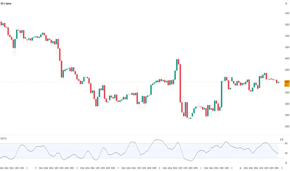
HTF BIAS FILTER🧭HTF Bias Filter Indicator: 5 in 1 indicator
Technical Overview
The Bias Filter is a comprehensive multi-timeframe tool designed to confirm directional bias using five key indicators before entering a trade. It plots higher-timeframe Moving Averages directly on the chart and provides an immediate status summary via a static dashboard.
The more confluence on the dashboard, the greater the probability of the direction of the trade.
1. 📊 Display Components
A. Plotted Lines
The indicator uses the request.security function to draw Moving Averages from higher timeframes onto your current chart:
1H EMA 21 (Purple): The 21-period Exponential Moving Average calculated on the 1-Hour (60 min) chart. Plotted using a step-line style.
4H EMA 50 (Red): The 50-period Exponential Moving Average calculated on the 4-Hour (240 min) chart. Plotted using a step-line style.
B. Directional Dashboard
A fixed-position summary table is anchored to the bottom-right corner of the chart, providing a quick glance at the current status of all five filters.
2. 🎨 Colour Logic
Each of the five indicators is assigned a colour based on its current directional signal. The more indicators that show the same colour (confluence), the stronger the signal and the higher the likelihood of a high-probability trade.
🟢 Green indicators are signaling UP/BUY (Bullish momentum or trend).
🔴 Red indicators are signaling DOWN/SELL (Bearish momentum or trend).
⚫ Gray indicators are signaling Mixed or flat directions (neutral or undecided).
Note: The dashboard's main header color is determined by a strict confluence logic (All four 4H filters must align for Green/Red), while individual indicator colors follow the simple rules above.
3. 📋 Indicator Breakdown and Logic
The dashboard provides the direction of five different filters.
3.1. Higher-Timeframe (HTF) Trend Indicators
These two signals determine the immediate slope and direction of the primary Moving Averages:
4H EMA 50:
Timeframe: 4-Hour (240 min)
Logic: Compares the current EMA value to the value two bars ago on the 4H chart.
Output: UP ↑, DOWN ↓, or FLAT ⏸
1H EMA 21:
Timeframe: 1-Hour (60 min)
Logic: Compares the current EMA value to the value two bars ago on the 1H chart.
Output: UP ↑, DOWN ↓, or FLAT ⏸
3.2. 4-Hour Confluence Filters
These three indicators provide supplementary confirmation on Volume, Price Position, and Momentum, all calculated on the 4-Hour (240 min) chart:
4H OBV (Smoothed):
Timeframe: 4-Hour (240 min)
Logic: Direction is based on the current value of the 21-bar smoothed On-Balance Volume (OBV) compared to its value nine bars ago.
Output: UP ↑, DOWN ↓, or FLAT ⏸
4H ATR DIR (EMA Proxy):
Timeframe: 4-Hour (240 min)
Logic: Determines the price position by comparing the current Close price against the 4H EMA 50.
Output: BUY 🟢 (Close > EMA 50), SELL 🔴 (Close < EMA 50), or FLAT ⏸️ (Close = EMA 50).
4H RSI (14):
Timeframe: 4-Hour (240 min)
Logic: Momentum check comparing the 14-period Relative Strength Index (RSI) value against the 50 level.
Output: BUY 🟢 (RSI > 50), SELL 🔴 (RSI < 50), or FLAT ⏸️ (RSI = 50).

SMC BOS/CHoCH + Auto Fib (5m/any TF) durane//@version=6
indicator('SMC BOS/CHoCH + Auto Fib (5m/any TF)', overlay = true, max_lines_count = 200, max_labels_count = 200)
// --------- Inputs ----------
left = input.int(3, 'Pivot Left', minval = 1)
right = input.int(3, 'Pivot Right', minval = 1)
minSwingSize = input.float(0.0, 'Min swing size (price units, 0 = disabled)', step = 0.1)
fib_levels = input.string('0.0,0.236,0.382,0.5,0.618,0.786,1.0', 'Fibonacci levels (comma separated)')
show_labels = input.bool(true, 'Show BOS/CHoCH labels')
lookbackHighLow = input.int(200, 'Lookback for structure (bars)')
// Parse fib levels
strs = str.split(fib_levels, ',')
var array fibs = array.new_float()
if barstate.isfirst
for s in strs
array.push(fibs, str.tonumber(str.trim(s)))
// --------- Find pivot highs / lows ----------
pHigh = ta.pivothigh(high, left, right)
pLow = ta.pivotlow(low, left, right)
// store last confirmed swings
var float lastSwingHighPrice = na
var int lastSwingHighBar = na
var float lastSwingLowPrice = na
var int lastSwingLowBar = na
if not na(pHigh)
// check min size
if minSwingSize == 0 or pHigh - nz(lastSwingLowPrice, pHigh) >= minSwingSize
lastSwingHighPrice := pHigh
lastSwingHighBar := bar_index - right
lastSwingHighBar
if not na(pLow)
if minSwingSize == 0 or nz(lastSwingHighPrice, pLow) - pLow >= minSwingSize
lastSwingLowPrice := pLow
lastSwingLowBar := bar_index - right
lastSwingLowBar
// --------- Detect BOS & CHoCH (simple robust logic) ----------
var int lastBOSdir = 0 // 1 = bullish BOS (price broke above), -1 = bearish BOS
var int lastBOSbar = na
var float lastBOSprice = na
// Look for price closes beyond last structural swings within lookback
// Bullish BOS: close > recent swing high
condBullBOS = not na(lastSwingHighPrice) and close > lastSwingHighPrice and bar_index - lastSwingHighBar <= lookbackHighLow
// Bearish BOS: close < recent swing low
condBearBOS = not na(lastSwingLowPrice) and close < lastSwingLowPrice and bar_index - lastSwingLowBar <= lookbackHighLow
bosTriggered = false
chochTriggered = false
if condBullBOS
bosTriggered := true
if lastBOSdir != 1
// if previous BOS direction was -1, this is CHoCH (change of character)
chochTriggered := lastBOSdir == -1
chochTriggered
lastBOSdir := 1
lastBOSbar := bar_index
lastBOSprice := close
lastBOSprice
if condBearBOS
bosTriggered := true
if lastBOSdir != -1
chochTriggered := lastBOSdir == 1
chochTriggered
lastBOSdir := -1
lastBOSbar := bar_index
lastBOSprice := close
lastBOSprice
// --------- Plot labels for BOS / CHoCH ----------
if bosTriggered and show_labels
if chochTriggered
label.new(bar_index, high, text = lastBOSdir == 1 ? 'CHoCH ↑' : 'CHoCH ↓', style = label.style_label_up, color = color.new(color.orange, 0), textcolor = color.white, yloc = yloc.abovebar)
else
label.new(bar_index, high, text = lastBOSdir == 1 ? 'BOS ↑' : 'BOS ↓', style = label.style_label_left, color = lastBOSdir == 1 ? color.green : color.red, textcolor = color.white, yloc = yloc.abovebar)
// --------- Auto Fibonacci drawing ----------
var array fib_lines = array.new_line()
var array fib_labels = array.new_label()
var int lastFibId = na
// Function to clear previous fibs
f_clear() =>
if array.size(fib_lines) > 0
for i = 0 to array.size(fib_lines) - 1
line.delete(array.get(fib_lines, i))
if array.size(fib_labels) > 0
for i = 0 to array.size(fib_labels) - 1
label.delete(array.get(fib_labels, i))
array.clear(fib_lines)
array.clear(fib_labels)
// Decide anchors for fib: if lastBOSdir==1 (bullish) anchor from lastSwingLow -> lastSwingHigh
// if lastBOSdir==-1 (bearish) anchor from lastSwingHigh -> lastSwingLow
if lastBOSdir == 1 and not na(lastSwingLowPrice) and not na(lastSwingHighPrice)
// bullish fib: low -> high
startPrice = lastSwingLowPrice
endPrice = lastSwingHighPrice
// draw
f_clear()
for i = 0 to array.size(fibs) - 1 by 1
lvl = array.get(fibs, i)
priceLevel = startPrice + (endPrice - startPrice) * lvl
ln = line.new(x1 = lastSwingLowBar, y1 = priceLevel, x2 = bar_index, y2 = priceLevel, xloc = xloc.bar_index, extend = extend.right, color = color.new(color.green, 60), width = 1, style = line.style_solid)
array.push(fib_lines, ln)
lab = label.new(bar_index, priceLevel, text = str.tostring(lvl * 100, '#.0') + '%', style = label.style_label_right, color = color.new(color.green, 80), textcolor = color.white, yloc = yloc.price)
array.push(fib_labels, lab)
if lastBOSdir == -1 and not na(lastSwingHighPrice) and not na(lastSwingLowPrice)
// bearish fib: high -> low
startPrice = lastSwingHighPrice
endPrice = lastSwingLowPrice
f_clear()
for i = 0 to array.size(fibs) - 1 by 1
lvl = array.get(fibs, i)
priceLevel = startPrice + (endPrice - startPrice) * lvl
ln = line.new(x1 = lastSwingHighBar, y1 = priceLevel, x2 = bar_index, y2 = priceLevel, xloc = xloc.bar_index, extend = extend.right, color = color.new(color.red, 60), width = 1, style = line.style_solid)
array.push(fib_lines, ln)
lab = label.new(bar_index, priceLevel, text = str.tostring(lvl * 100, '#.0') + '%', style = label.style_label_right, color = color.new(color.red, 80), textcolor = color.white, yloc = yloc.price)
array.push(fib_labels, lab)
// --------- Optional: plot lastSwing points ----------
plotshape(not na(lastSwingHighPrice) ? lastSwingHighPrice : na, title = 'LastSwingHigh', location = location.absolute, style = shape.triangledown, size = size.tiny, color = color.red, offset = 0)
plotshape(not na(lastSwingLowPrice) ? lastSwingLowPrice : na, title = 'LastSwingLow', location = location.absolute, style = shape.triangleup, size = size.tiny, color = color.green, offset = 0)
// --------- Alerts ----------
alertcondition(bosTriggered and lastBOSdir == 1, title = 'Bullish BOS', message = 'Bullish BOS detected on {{ticker}} @ {{close}}')
alertcondition(bosTriggered and lastBOSdir == -1, title = 'Bearish BOS', message = 'Bearish BOS detected on {{ticker}} @ {{close}}')
alertcondition(chochTriggered, title = 'CHoCH Detected', message = 'CHoCH detected on {{ticker}} @ {{close}}')
// End
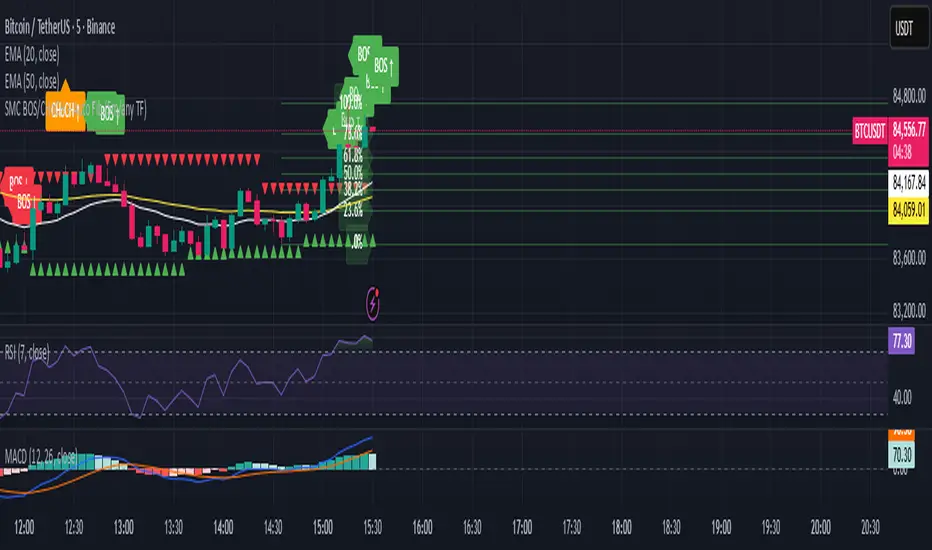
coinjin 정·역배열 대시보드 (Progress+Events)This script analyzes trend alignment using the 5 / 20 / 60 / 112 / 224 / 448 / 896 SMAs,
providing highly precise detection of bullish and bearish stack conditions,
and identifies 12 advanced trend-reversal signals through a multi-timeframe dashboard.
이 스크립트는 5 / 20 / 60 / 112 / 224 / 448 / 896 SMA 기준으로
정배열·역배열 상태를 매우 정교하게 분석하고,
12가지 고급 추세 전환 시그널을 자동 탐지하는 멀티타임프레임 대시보드입니다.

Scout Regiment - KSI# Scout Regiment - KSI Indicator
## English Documentation
### Overview
Scout Regiment - KSI (Key Stochastic Indicators) is a comprehensive momentum oscillator that combines three powerful technical indicators - RSI, CCI, and Williams %R - into a single, unified display. This multi-indicator approach provides traders with diverse perspectives on market momentum, overbought/oversold conditions, and potential reversal points through advanced divergence detection.
### What is KSI?
KSI stands for "Key Stochastic Indicators" - a composite momentum indicator that:
- Displays multiple oscillators normalized to a 0-100 scale
- Uses standardized bands (20/50/80) for consistent interpretation
- Combines RSI for trend, CCI for cycle, and Williams %R for reversal detection
- Provides enhanced divergence detection specifically for RSI
### Key Features
#### 1. **Triple Oscillator System**
**① RSI (Relative Strength Index)** - Primary Indicator
- **Purpose**: Measures momentum and identifies overbought/oversold conditions
- **Default Length**: 22 periods
- **Display**: Blue line (2px)
- **Key Levels**:
- Above 50: Bullish momentum
- Below 50: Bearish momentum
- Above 80: Overbought
- Below 20: Oversold
- **Special Features**:
- Background color indication (green/red)
- Crossover labels at 50 level
- Full divergence detection (4 types)
**② CCI (Commodity Channel Index)** - Dual Period
- **Purpose**: Identifies cyclical trends and extreme conditions
- **Dual Display**:
- CCI(33): Short-term cycle - Green line (1px)
- CCI(77): Medium-term cycle - Orange line (1px)
- **Default Source**: HLC3 (typical price)
- **Normalized Scale**: Mapped from ±100 to 0-100 for consistency
- **Interpretation**:
- Above 80: Strong upward momentum
- Below 20: Strong downward momentum
- 50 level: Neutral
- Divergence between periods: Trend change warning
**③ Williams %R** - Optional
- **Purpose**: Identifies overbought/oversold extremes
- **Default Length**: 28 periods
- **Display**: Magenta line (2px)
- **Scale**: Inverted and normalized to 0-100
- **Best For**: Short-term reversal signals
- **Default**: Disabled (enable when needed for extra confirmation)
#### 2. **Standardized Band System**
**Three-Level Structure:**
- **Upper Band (80)**: Overbought zone
- Strong momentum area
- Watch for reversal signals
- Divergences here are most reliable
- **Middle Line (50)**: Equilibrium
- Separates bullish/bearish zones
- Crossovers indicate momentum shifts
- Key decision level
- **Lower Band (20)**: Oversold zone
- Weak momentum area
- Look for bounce signals
- Divergences here signal potential reversals
**Band Fill**: Dark background between 20-80 for visual clarity
#### 3. **RSI Visual Enhancements**
**Background Color Indication**
- Green background: RSI above 50 (bullish bias)
- Red background: RSI below 50 (bearish bias)
- Optional display for cleaner charts
- Helps identify overall momentum direction
**Crossover Labels**
- "突破" (Breakout): RSI crosses above 50
- "跌破" (Breakdown): RSI crosses below 50
- Marks momentum shift points
- Can be toggled on/off
#### 4. **Advanced RSI Divergence Detection**
The indicator includes comprehensive divergence detection for RSI only (most reliable oscillator):
**Regular Bullish Divergence (Yellow)**
- **Price**: Lower lows
- **RSI**: Higher lows
- **Signal**: Potential upward reversal
- **Label**: "涨" (Up)
- **Most Common**: Near oversold levels (below 30)
**Regular Bearish Divergence (Blue)**
- **Price**: Higher highs
- **RSI**: Lower highs
- **Signal**: Potential downward reversal
- **Label**: "跌" (Down)
- **Most Common**: Near overbought levels (above 70)
**Hidden Bullish Divergence (Light Yellow)**
- **Price**: Higher lows
- **RSI**: Lower lows
- **Signal**: Uptrend continuation
- **Label**: "隐涨" (Hidden Up)
- **Use**: Add to existing longs
**Hidden Bearish Divergence (Light Blue)**
- **Price**: Lower highs
- **RSI**: Higher highs
- **Signal**: Downtrend continuation
- **Label**: "隐跌" (Hidden Down)
- **Use**: Add to existing shorts
**Divergence Parameters** (Fully Customizable):
- **Right Lookback**: Bars to right of pivot (default: 5)
- **Left Lookback**: Bars to left of pivot (default: 5)
- **Max Range**: Maximum bars between pivots (default: 60)
- **Min Range**: Minimum bars between pivots (default: 5)
### Configuration Settings
#### KSI Display Settings
- **Show RSI**: Toggle RSI indicator
- **Show CCI**: Toggle both CCI lines
- **Show Williams %R**: Toggle Williams %R (optional)
#### RSI Settings
- **RSI Length**: Period for calculation (default: 22)
- **Data Source**: Price source (default: close)
- **Show Background**: Toggle green/red background
- **Show Cross Labels**: Toggle 50-level crossover labels
#### RSI Divergence Settings
- **Right Lookback**: Pivot detection right side
- **Left Lookback**: Pivot detection left side
- **Max Range**: Maximum lookback distance
- **Min Range**: Minimum lookback distance
- **Show Regular Divergence**: Enable regular divergence lines
- **Show Regular Labels**: Enable regular divergence labels
- **Show Hidden Divergence**: Enable hidden divergence lines
- **Show Hidden Labels**: Enable hidden divergence labels
#### CCI Settings
- **CCI Length**: Short-term period (default: 33)
- **CCI Mid Length**: Medium-term period (default: 77)
- **Data Source**: Price calculation (default: HLC3)
- **Show CCI(33)**: Toggle short-term CCI
- **Show CCI(77)**: Toggle medium-term CCI
#### Williams %R Settings
- **Length**: Calculation period (default: 28)
- **Data Source**: Price source (default: close)
### How to Use
#### For Basic Momentum Trading
1. **Enable RSI Only** (primary indicator)
- Focus on 50-level crossovers
- Enable crossover labels for signals
2. **Identify Momentum Direction**
- RSI > 50 = Bullish momentum
- RSI < 50 = Bearish momentum
- Background color confirms direction
3. **Look for Extremes**
- RSI > 80 = Overbought (consider selling)
- RSI < 20 = Oversold (consider buying)
4. **Trade Setup**
- Enter long when RSI crosses above 50 from oversold
- Enter short when RSI crosses below 50 from overbought
#### For Divergence Trading
1. **Enable RSI with Divergence Detection**
- Turn on regular divergence
- Optionally add hidden divergence
2. **Wait for Divergence Signal**
- Yellow label = Bullish divergence
- Blue label = Bearish divergence
3. **Confirm with Price Structure**
- Wait for support/resistance break
- Look for candlestick patterns
- Check volume confirmation
4. **Enter Position**
- Enter after confirmation
- Stop beyond divergence pivot
- Target next key level
#### For Multi-Oscillator Confirmation
1. **Enable All Three Indicators**
- RSI (momentum)
- CCI dual (cycle analysis)
- Williams %R (extremes)
2. **Look for Alignment**
- All above 50 = Strong bullish
- All below 50 = Strong bearish
- Mixed signals = Consolidation
3. **Identify Extremes**
- All indicators > 80 = Extreme overbought
- All indicators < 20 = Extreme oversold
4. **Trade Reversals**
- Enter counter-trend when all aligned at extremes
- Confirm with divergence if available
- Use tight stops
#### For CCI Dual-Period Analysis
1. **Enable Both CCI Lines**
- CCI(33) = Short-term
- CCI(77) = Medium-term
2. **Watch for Crossovers**
- Green crosses above orange = Bullish acceleration
- Green crosses below orange = Bearish acceleration
3. **Analyze Divergence Between Periods**
- Short-term rising, medium falling = Potential reversal
- Both rising together = Strong trend
4. **Trade Accordingly**
- Follow crossover direction
- Exit when lines converge
### Trading Strategies
#### Strategy 1: RSI 50-Level Crossover
**Setup:**
- Enable RSI with background and labels
- Wait for clear trend
- Look for retracement to 50 level
**Entry:**
- Long: "突破" label appears after pullback
- Short: "跌破" label appears after bounce
**Stop Loss:**
- Long: Below recent swing low
- Short: Above recent swing high
**Exit:**
- Opposite crossover label
- Or predetermined target (2:1 risk-reward)
**Best For:** Trend following, clear markets
#### Strategy 2: RSI Divergence Reversal
**Setup:**
- Enable RSI with regular divergence
- Wait for extreme levels (>70 or <30)
- Look for divergence signal
**Entry:**
- Long: Yellow "涨" label at oversold level
- Short: Blue "跌" label at overbought level
**Confirmation:**
- Wait for price to break structure
- Check for volume increase
- Look for candlestick reversal pattern
**Stop Loss:**
- Beyond divergence pivot point
**Exit:**
- Take partial profit at 50 level
- Exit remainder at opposite extreme or divergence
**Best For:** Swing trading, range-bound markets
#### Strategy 3: Triple Oscillator Confluence
**Setup:**
- Enable all three indicators
- Wait for all to reach extreme (>80 or <20)
- Look for alignment
**Entry:**
- Long: All three below 20, first one crosses above 20
- Short: All three above 80, first one crosses below 80
**Confirmation:**
- All indicators must align
- Price at support/resistance
- Volume spike helps
**Stop Loss:**
- Fixed percentage or ATR-based
**Exit:**
- When any indicator crosses 50 level
- Or at predetermined target
**Best For:** High-probability reversals, volatile markets
#### Strategy 4: CCI Dual-Period System
**Setup:**
- Enable both CCI lines only
- Disable RSI and Williams %R for clarity
- Watch for crossovers
**Entry:**
- Long: CCI(33) crosses above CCI(77) below 50 line
- Short: CCI(33) crosses below CCI(77) above 50 line
**Confirmation:**
- Both should be moving in entry direction
- Price breaking key level helps
**Stop Loss:**
- When CCIs cross back in opposite direction
**Exit:**
- Both CCIs enter opposite extreme zone
- Or trailing stop
**Best For:** Catching trend continuations, momentum trading
#### Strategy 5: Hidden Divergence Continuation
**Setup:**
- Enable RSI with hidden divergence
- Confirm existing trend
- Wait for pullback
**Entry:**
- Uptrend: "隐涨" label during pullback
- Downtrend: "隐跌" label during bounce
**Confirmation:**
- Price holds key moving average
- Trend structure intact
**Stop Loss:**
- Beyond pullback extreme
**Exit:**
- Regular divergence appears (reversal warning)
- Or trend structure breaks
**Best For:** Adding to positions, trend trading
### Best Practices
#### Choosing Which Indicators to Display
**For Beginners:**
- Use RSI only
- Enable background color and labels
- Focus on 50-level crossovers
- Simple and effective
**For Intermediate Traders:**
- RSI + Regular Divergence
- Add CCI for confirmation
- Use dual perspectives
- Better accuracy
**For Advanced Traders:**
- All three indicators
- Full divergence detection
- Multi-timeframe analysis
- Maximum information
#### Oscillator Priority
**Primary**: RSI (22)
- Most reliable
- Best divergence detection
- Good for all timeframes
- Use this as your main decision maker
**Secondary**: CCI (33/77)
- Adds cycle analysis
- Great for confirmation
- Dual-period crossovers valuable
- Use to confirm RSI signals
**Tertiary**: Williams %R (28)
- Extreme readings useful
- More volatile
- Best for short-term
- Use sparingly for extra confirmation
#### Timeframe Considerations
**Lower Timeframes (1m-15m):**
- More signals, less reliable
- Use tight divergence parameters
- Focus on RSI crossovers
- Quick entries and exits
**Medium Timeframes (30m-4H):**
- Balanced signal frequency
- Default settings work well
- Best for divergence trading
- Swing trading optimal
**Higher Timeframes (Daily+):**
- Fewer but stronger signals
- Widen divergence ranges
- All indicators more reliable
- Position trading best
#### Divergence Trading Tips
1. **Wait for Confirmation**
- Divergence alone isn't enough
- Need price structure break
- Volume helps validate
2. **Best at Extremes**
- Divergences near 80/20 levels most reliable
- Mid-level divergences often fail
- Combine with support/resistance
3. **Multiple Divergences**
- Second divergence stronger than first
- Third divergence extremely powerful
- Watch for "triple divergence"
4. **Timeframe Alignment**
- Check higher timeframe for direction
- Trade divergences in direction of larger trend
- Counter-trend divergences riskier
### Indicator Combinations
**With Moving Averages:**
- Use EMAs (21/55/144) for trend
- KSI for entry timing
- Enter when both align
**With Volume:**
- Volume confirms breakouts
- Divergence + volume divergence = Stronger
- Low volume at extremes = Reversal likely
**With Support/Resistance:**
- Price levels for targets
- KSI for entry timing
- Divergences at levels = Highest probability
**With Bias Indicator:**
- Bias shows price deviation
- KSI shows momentum
- Both diverging = Strong reversal signal
**With OBV Indicator:**
- OBV shows volume trend
- KSI shows price momentum
- Volume/momentum divergence powerful
### Common Patterns
1. **Bullish Reversal**: All oscillators oversold + RSI bullish divergence
2. **Bearish Reversal**: All oscillators overbought + RSI bearish divergence
3. **Trend Acceleration**: RSI > 50, both CCIs rising, Williams %R not extreme
4. **Weakening Trend**: RSI declining while price rising (pre-divergence warning)
5. **Strong Trend**: All oscillators stay above/below 50 for extended period
6. **Consolidation**: Oscillators crossing 50 frequently without extremes
7. **Exhaustion**: Multiple oscillators at extreme + hidden divergence failure
### Performance Tips
- Start simple: RSI only
- Add indicators gradually as you learn
- Disable unused features for cleaner charts
- Use labels strategically (not always on)
- Test different RSI lengths for your market
- Adjust divergence parameters based on volatility
### Alert Conditions
The indicator includes alerts for:
- RSI crossing above 50
- RSI crossing below 50
- RSI regular bullish divergence
- RSI regular bearish divergence
- RSI hidden bullish divergence
- RSI hidden bearish divergence
---
## 中文说明文档
### 概述
Scout Regiment - KSI(关键随机指标)是一个综合性动量振荡器,将三个强大的技术指标 - RSI、CCI和威廉指标 - 组合到一个统一的显示中。这种多指标方法为交易者提供了市场动量、超买超卖状况和通过高级背离检测发现潜在反转点的多元视角。
### 什么是KSI?
KSI代表"关键随机指标" - 一个综合动量指标:
- 显示多个振荡器,标准化到0-100刻度
- 使用标准化波段(20/50/80)便于一致解读
- 结合RSI用于趋势、CCI用于周期、威廉指标用于反转检测
- 专门为RSI提供增强的背离检测
### 核心功能
#### 1. **三重振荡器系统**
**① RSI(相对强弱指数)** - 主要指标
- **用途**:测量动量并识别超买超卖状况
- **默认长度**:22周期
- **显示**:蓝色线(2像素)
- **关键水平**:
- 50以上:看涨动量
- 50以下:看跌动量
- 80以上:超买
- 20以下:超卖
- **特殊功能**:
- 背景颜色指示(绿色/红色)
- 50水平穿越标签
- 完整背离检测(4种类型)
**② CCI(顺势指标)** - 双周期
- **用途**:识别周期性趋势和极端状况
- **双重显示**:
- CCI(33):短期周期 - 绿色线(1像素)
- CCI(77):中期周期 - 橙色线(1像素)
- **默认数据源**:HLC3(典型价格)
- **标准化刻度**:从±100映射到0-100以保持一致性
- **解读**:
- 80以上:强劲上升动量
- 20以下:强劲下降动量
- 50水平:中性
- 周期间背离:趋势变化警告
**③ 威廉指标 %R** - 可选
- **用途**:识别超买超卖极值
- **默认长度**:28周期
- **显示**:洋红色线(2像素)
- **刻度**:反转并标准化到0-100
- **最适合**:短期反转信号
- **默认**:禁用(需要额外确认时启用)
#### 2. **标准化波段系统**
**三层结构:**
- **上轨(80)**:超买区域
- 强动量区域
- 注意反转信号
- 此处的背离最可靠
- **中线(50)**:均衡线
- 分隔看涨/看跌区域
- 穿越表示动量转变
- 关键决策水平
- **下轨(20)**:超卖区域
- 弱动量区域
- 寻找反弹信号
- 此处的背离预示潜在反转
**波段填充**:20-80之间的深色背景,增强视觉清晰度
#### 3. **RSI视觉增强**
**背景颜色指示**
- 绿色背景:RSI在50以上(看涨偏向)
- 红色背景:RSI在50以下(看跌偏向)
- 可选显示,图表更清爽
- 帮助识别整体动量方向
**穿越标签**
- "突破":RSI向上穿越50
- "跌破":RSI向下穿越50
- 标记动量转变点
- 可开关
#### 4. **高级RSI背离检测**
指标仅为RSI(最可靠的振荡器)提供全面背离检测:
**常规看涨背离(黄色)**
- **价格**:更低的低点
- **RSI**:更高的低点
- **信号**:潜在向上反转
- **标签**:"涨"
- **最常见**:在超卖水平附近(30以下)
**常规看跌背离(蓝色)**
- **价格**:更高的高点
- **RSI**:更低的高点
- **信号**:潜在向下反转
- **标签**:"跌"
- **最常见**:在超买水平附近(70以上)
**隐藏看涨背离(浅黄色)**
- **价格**:更高的低点
- **RSI**:更低的低点
- **信号**:上升趋势延续
- **标签**:"隐涨"
- **用途**:加仓现有多头
**隐藏看跌背离(浅蓝色)**
- **价格**:更低的高点
- **RSI**:更高的高点
- **信号**:下降趋势延续
- **标签**:"隐跌"
- **用途**:加仓现有空头
**背离参数**(完全可自定义):
- **右侧回溯**:枢轴点右侧K线数(默认:5)
- **左侧回溯**:枢轴点左侧K线数(默认:5)
- **最大范围**:枢轴点之间最大K线数(默认:60)
- **最小范围**:枢轴点之间最小K线数(默认:5)
### 配置设置
#### KSI显示设置
- **显示RSI**:切换RSI指标
- **显示CCI**:切换两条CCI线
- **显示威廉指标 %R**:切换威廉指标(可选)
#### RSI设置
- **RSI长度**:计算周期(默认:22)
- **数据源**:价格源(默认:收盘价)
- **显示背景**:切换绿色/红色背景
- **显示穿越标签**:切换50水平穿越标签
#### RSI背离设置
- **右侧回溯**:枢轴检测右侧
- **左侧回溯**:枢轴检测左侧
- **回溯范围最大值**:最大回溯距离
- **回溯范围最小值**:最小回溯距离
- **显示常规背离**:启用常规背离线
- **显示常规背离标签**:启用常规背离标签
- **显示隐藏背离**:启用隐藏背离线
- **显示隐藏背离标签**:启用隐藏背离标签
#### CCI设置
- **CCI长度**:短期周期(默认:33)
- **CCI中期长度**:中期周期(默认:77)
- **数据源**:价格计算(默认:HLC3)
- **显示CCI(33)**:切换短期CCI
- **显示CCI(77)**:切换中期CCI
#### 威廉指标 %R 设置
- **长度**:计算周期(默认:28)
- **数据源**:价格源(默认:收盘价)
### 使用方法
#### 基础动量交易
1. **仅启用RSI**(主要指标)
- 关注50水平穿越
- 启用穿越标签获取信号
2. **识别动量方向**
- RSI > 50 = 看涨动量
- RSI < 50 = 看跌动量
- 背景颜色确认方向
3. **寻找极值**
- RSI > 80 = 超买(考虑卖出)
- RSI < 20 = 超卖(考虑买入)
4. **交易设置**
- RSI从超卖区向上穿越50时做多
- RSI从超买区向下穿越50时做空
#### 背离交易
1. **启用RSI和背离检测**
- 打开常规背离
- 可选添加隐藏背离
2. **等待背离信号**
- 黄色标签 = 看涨背离
- 蓝色标签 = 看跌背离
3. **用价格结构确认**
- 等待支撑/阻力突破
- 寻找K线形态
- 检查成交量确认
4. **进入仓位**
- 确认后进入
- 止损设在背离枢轴点之外
- 目标下一个关键水平
#### 多振荡器确认
1. **启用全部三个指标**
- RSI(动量)
- CCI双周期(周期分析)
- 威廉指标 %R(极值)
2. **寻找一致性**
- 全部在50以上 = 强劲看涨
- 全部在50以下 = 强劲看跌
- 信号混合 = 盘整
3. **识别极值**
- 所有指标 > 80 = 极度超买
- 所有指标 < 20 = 极度超卖
4. **交易反转**
- 所有指标在极值一致时逆势进入
- 可能的话用背离确认
- 使用紧密止损
#### CCI双周期分析
1. **启用两条CCI线**
- CCI(33) = 短期
- CCI(77) = 中期
2. **观察穿越**
- 绿色线穿越橙色线向上 = 看涨加速
- 绿色线穿越橙色线向下 = 看跌加速
3. **分析周期间背离**
- 短期上升,中期下降 = 潜在反转
- 两者同时上升 = 强趋势
4. **相应交易**
- 跟随穿越方向
- 线条汇合时退出
### 交易策略
#### 策略1:RSI 50水平穿越
**设置:**
- 启用RSI及背景和标签
- 等待明确趋势
- 寻找回调至50水平
**入场:**
- 多头:回调后出现"突破"标签
- 空头:反弹后出现"跌破"标签
**止损:**
- 多头:近期波动低点之下
- 空头:近期波动高点之上
**离场:**
- 出现相反穿越标签
- 或预定目标(2:1风险收益比)
**适合:**趋势跟随、明确市场
#### 策略2:RSI背离反转
**设置:**
- 启用RSI和常规背离
- 等待极端水平(>70或<30)
- 寻找背离信号
**入场:**
- 多头:超卖水平出现黄色"涨"标签
- 空头:超买水平出现蓝色"跌"标签
**确认:**
- 等待价格突破结构
- 检查成交量增加
- 寻找K线反转形态
**止损:**
- 背离枢轴点之外
**离场:**
- 在50水平部分获利
- 其余在相反极值或背离处离场
**适合:**波段交易、震荡市场
#### 策略3:三重振荡器汇合
**设置:**
- 启用全部三个指标
- 等待全部达到极值(>80或<20)
- 寻找一致性
**入场:**
- 多头:三个全部低于20,第一个向上穿越20
- 空头:三个全部高于80,第一个向下穿越80
**确认:**
- 所有指标必须一致
- 价格在支撑/阻力位
- 成交量激增有帮助
**止损:**
- 固定百分比或基于ATR
**离场:**
- 任一指标穿越50水平时
- 或在预定目标
**适合:**高概率反转、波动市场
#### 策略4:CCI双周期系统
**设置:**
- 仅启用两条CCI线
- 禁用RSI和威廉指标以保持清晰
- 观察穿越
**入场:**
- 多头:CCI(33)在50线下方向上穿越CCI(77)
- 空头:CCI(33)在50线上方向下穿越CCI(77)
**确认:**
- 两者都应朝入场方向移动
- 价格突破关键水平有帮助
**止损:**
- CCI反向穿越时
**离场:**
- 两条CCI进入相反极值区域
- 或移动止损
**适合:**捕捉趋势延续、动量交易
#### 策略5:隐藏背离延续
**设置:**
- 启用RSI和隐藏背离
- 确认现有趋势
- 等待回调
**入场:**
- 上升趋势:回调期间出现"隐涨"标签
- 下降趋势:反弹期间出现"隐跌"标签
**确认:**
- 价格守住关键移动平均线
- 趋势结构完整
**止损:**
- 回调极值之外
**离场:**
- 出现常规背离(反转警告)
- 或趋势结构破坏
**适合:**加仓、趋势交易
### 最佳实践
#### 选择显示哪些指标
**新手:**
- 仅使用RSI
- 启用背景颜色和标签
- 关注50水平穿越
- 简单有效
**中级交易者:**
- RSI + 常规背离
- 添加CCI确认
- 使用双重视角
- 更高准确度
**高级交易者:**
- 全部三个指标
- 完整背离检测
- 多时间框架分析
- 信息最大化
#### 振荡器优先级
**主要**:RSI (22)
- 最可靠
- 最佳背离检测
- 适用所有时间框架
- 用作主要决策依据
**次要**:CCI (33/77)
- 添加周期分析
- 确认效果好
- 双周期穿越有价值
- 用于确认RSI信号
**第三**:威廉指标 %R (28)
- 极值读数有用
- 更波动
- 最适合短期
- 谨慎使用以获额外确认
#### 时间框架考虑
**低时间框架(1分钟-15分钟):**
- 更多信号,可靠性较低
- 使用紧密背离参数
- 关注RSI穿越
- 快速进出
**中等时间框架(30分钟-4小时):**
- 信号频率平衡
- 默认设置效果好
- 最适合背离交易
- 波段交易最优
**高时间框架(日线+):**
- 信号较少但更强
- 扩大背离范围
- 所有指标更可靠
- 最适合仓位交易
#### 背离交易技巧
1. **等待确认**
- 仅背离不够
- 需要价格结构突破
- 成交量帮助验证
2. **极值处最佳**
- 80/20水平附近的背离最可靠
- 中间水平背离常失败
- 结合支撑/阻力
3. **多重背离**
- 第二次背离强于第一次
- 第三次背离极其强大
- 注意"三重背离"
4. **时间框架对齐**
- 检查更高时间框架方向
- 顺大趋势方向交易背离
- 逆势背离风险更大
### 指标组合
**与移动平均线配合:**
- 使用EMA(21/55/144)确定趋势
- KSI用于入场时机
- 两者一致时进入
**与成交量配合:**
- 成交量确认突破
- 背离 + 成交量背离 = 更强
- 极值处低成交量 = 可能反转
**与支撑/阻力配合:**
- 价格水平作为目标
- KSI用于入场时机
- 水平处的背离 = 最高概率
**与Bias指标配合:**
- Bias显示价格偏离
- KSI显示动量
- 两者都背离 = 强反转信号
**与OBV指标配合:**
- OBV显示成交量趋势
- KSI显示价格动量
- 成交量/动量背离强大
### 常见形态
1. **看涨反转**:所有振荡器超卖 + RSI看涨背离
2. **看跌反转**:所有振荡器超买 + RSI看跌背离
3. **趋势加速**:RSI > 50,两条CCI上升,威廉指标不极端
4. **趋势减弱**:价格上升时RSI下降(背离前警告)
5. **强趋势**:所有振荡器长时间保持在50上方/下方
6. **盘整**:振荡器频繁穿越50无极值
7. **衰竭**:多个振荡器在极值 + 隐藏背离失败
### 性能提示
- 从简单开始:仅RSI
- 学习时逐渐添加指标
- 禁用未使用功能以保持图表清晰
- 策略性使用标签(不总是开启)
- 为您的市场测试不同RSI长度
- 根据波动性调整背离参数
### 警报条件
指标包含以下警报:
- RSI向上穿越50
- RSI向下穿越50
- RSI常规看涨背离
- RSI常规看跌背离
- RSI隐藏看涨背离
- RSI隐藏看跌背离
---
## Technical Support
For questions or issues, please refer to the TradingView community or contact the indicator creator.
## 技术支持
如有问题,请参考TradingView社区或联系指标创建者。

Scout Regiment - Bias# Scout Regiment - Bias Indicator
## English Documentation
### Overview
Scout Regiment - Bias is a technical indicator that measures the deviation (bias) between the current price and exponential moving averages (EMAs). It helps traders identify overbought/oversold conditions, trend strength, and potential reversal points through divergence detection.
### What is Bias?
Bias measures how far the price has moved away from a moving average, expressed as a percentage:
- **Positive Bias**: Price is above the EMA (potential overbought)
- **Negative Bias**: Price is below the EMA (potential oversold)
- **Formula**: Bias = (Price - EMA) / EMA × 100
### Key Features
#### 1. **Triple EMA Bias Lines**
The indicator calculates bias from three different EMAs:
- **EMA 55 Bias** (Default: Green/Red, 1px line)
- Short-term bias measurement
- Quick response to price changes
- Best for intraday and swing trading
- **EMA 144 Bias** (Pink, 2px line)
- Medium-term bias measurement
- Balanced response to price movements
- Ideal for swing trading
- **EMA 233 Bias** (White, 2px line)
- Long-term bias measurement
- Slower response, more stable
- Best for position trading
**Color Coding:**
- Green: Price above EMA (bullish)
- Red: Price below EMA (bearish)
#### 2. **Visual Components**
**Histogram Display**
- Shows EMA 55 bias as a histogram for easy visualization
- Green bars: Price above EMA 55
- Red bars: Price below EMA 55
- Can be toggled on/off
**Background Color**
- Light green background: Bullish bias (price above EMA 55)
- Light red background: Bearish bias (price below EMA 55)
- Optional display for cleaner charts
**Zero Line**
- White horizontal line at 0%
- Reference point for positive/negative bias
- Crossovers indicate trend changes
**Crossover Labels**
- "突破" (Breakout): When bias crosses above zero
- "跌破" (Breakdown): When bias crosses below zero
- Can be enabled/disabled for clarity
#### 3. **Divergence Detection**
The indicator automatically detects regular divergences for all three bias lines:
**Bullish Divergence (Yellow Labels)**
- Price makes lower lows
- Bias makes higher lows
- Suggests potential upward reversal
- Labels: "55涨", "144涨", "233涨"
**Bearish Divergence (Blue Labels)**
- Price makes higher highs
- Bias makes lower highs
- Suggests potential downward reversal
- Labels: "55跌", "144跌", "233跌"
**Divergence Parameters** (Customizable for each EMA):
- Left Lookback: Bars to the left of pivot (default: 5)
- Right Lookback: Bars to the right of pivot (default: 1)
- Max Lookback Range: Maximum distance between pivots (default: 60)
- Min Lookback Range: Minimum distance between pivots (default: 5)
### Configuration Settings
#### Bias Settings
- **EMA Periods**: Customize lengths for EMA 55, 144, and 233
- **Price Source**: Choose calculation source (default: close)
- **Enable/Disable**: Toggle each bias line independently
#### Display Settings
- **Show Histogram**: Toggle histogram display
- **Show Background Color**: Toggle background coloring
- **Show Crossover Labels**: Toggle breakout/breakdown labels
#### Divergence Settings (Per EMA)
- Individual controls for EMA 55, 144, and 233 divergences
- Customizable lookback parameters for precision tuning
- Adjustable range settings for different market conditions
### How to Use
#### For Trend Trading
1. **Identify Trend Direction**
- Price above zero = Uptrend
- Price below zero = Downtrend
2. **Confirm with Multiple Timeframes**
- EMA 55: Short-term trend
- EMA 144: Medium-term trend
- EMA 233: Long-term trend
3. **Trade in Direction of Bias**
- All three lines positive = Strong uptrend
- All three lines negative = Strong downtrend
#### For Mean Reversion Trading
1. **Identify Extremes**
- High positive bias (>5-10%) = Overbought
- High negative bias (<-5 to -10%) = Oversold
2. **Wait for Confirmation**
- Look for bias to turn back toward zero
- Watch for crossover labels
3. **Enter on Reversal**
- Enter long when extreme negative bias starts rising
- Enter short when extreme positive bias starts falling
#### For Divergence Trading
1. **Spot Divergence Labels**
- Yellow labels = Bullish divergence (potential buy)
- Blue labels = Bearish divergence (potential sell)
2. **Confirm with Price Action**
- Wait for price to confirm with structure break
- Look for support/resistance reactions
3. **Use Multiple EMAs**
- EMA 55 divergence: Quick reversals
- EMA 144 divergence: Reliable signals
- EMA 233 divergence: Major trend changes
#### For Multi-Timeframe Analysis
1. **Check Long-term Bias** (EMA 233)
- Determines overall market direction
2. **Find Medium-term Entry** (EMA 144)
- Look for pullbacks in long-term trend
3. **Time Short-term Entry** (EMA 55)
- Enter when short-term aligns with longer timeframes
### Trading Strategies
#### Strategy 1: Triple Confirmation
- Wait for all three bias lines to be positive (or negative)
- Enter in direction of unanimous bias
- Exit when any line crosses zero
- Best for: Strong trending markets
#### Strategy 2: Divergence Trading
- Enable all divergence detection
- Take trades only when divergence appears
- Confirm with price structure
- Best for: Range-bound and reversal setups
#### Strategy 3: Zero Line Crossover
- Enable crossover labels
- Enter long on "突破" labels
- Enter short on "跌破" labels
- Use stop loss at recent swing points
- Best for: Trend following
#### Strategy 4: Extreme Reversion
- Wait for bias to reach extremes (>10% or <-10%)
- Enter counter-trend when bias reverses
- Exit at zero line
- Best for: Ranging markets
### Best Practices
1. **Combine with Price Action**
- Don't trade bias alone
- Confirm with support/resistance
- Look for candlestick patterns
2. **Use Multiple Timeframes**
- Check higher timeframe bias
- Trade in direction of larger trend
- Use lower timeframe for entry timing
3. **Manage Risk**
- Set stop losses beyond recent swings
- Don't fight extreme bias in strong trends
- Reduce position size at extremes
4. **Customize for Your Market**
- Volatile assets: Use wider ranges
- Stable assets: Use tighter ranges
- Adjust EMA periods for your timeframe
5. **Watch for False Signals**
- Multiple small divergences = Less reliable
- Divergences at extremes = More reliable
- Confirm with other indicators
### Indicator Combinations
**With Volume:**
- High bias + Low volume = Weak move
- High bias + High volume = Strong move
**With Moving Averages:**
- Check if price is above/below key EMAs
- Bias confirms EMA trend strength
**With RSI/MACD:**
- Multiple indicator divergence = Stronger signal
- Use bias for overbought/oversold confirmation
### Performance Tips
- Disable unused features for faster loading
- Use histogram for quick visual reference
- Enable background color for trend clarity
- Use divergence detection selectively
### Common Patterns
1. **Bias Expansion**: Bias increasing = Strong trend
2. **Bias Contraction**: Bias decreasing = Trend weakening
3. **Zero Line Bounce**: Price respects EMA as support/resistance
4. **Extreme Bias**: Over-extension, watch for reversal
5. **Divergence Cluster**: Multiple EMAs diverging = High probability reversal
### Alert Conditions
You can set alerts for:
- Bias crossing above/below zero
- Extreme bias levels
- Divergence detection
- All three bias lines aligned
---
## 中文说明文档
### 概述
Scout Regiment - Bias 是一个技术指标,用于测量当前价格与指数移动平均线(EMA)之间的偏离程度(乖离率)。它帮助交易者识别超买超卖状况、趋势强度,以及通过背离检测发现潜在的反转点。
### 什么是乖离率?
乖离率衡量价格偏离移动平均线的程度,以百分比表示:
- **正乖离**:价格高于EMA(可能超买)
- **负乖离**:价格低于EMA(可能超卖)
- **计算公式**:乖离率 = (价格 - EMA) / EMA × 100
### 核心功能
#### 1. **三重EMA乖离率线**
指标计算三条不同EMA的乖离率:
- **EMA 55 乖离率**(默认:绿色/红色,1像素线)
- 短期乖离测量
- 对价格变化反应快速
- 适合日内和波段交易
- **EMA 144 乖离率**(粉色,2像素线)
- 中期乖离测量
- 对价格波动反应平衡
- 最适合波段交易
- **EMA 233 乖离率**(白色,2像素线)
- 长期乖离测量
- 反应较慢,更稳定
- 适合仓位交易
**颜色编码:**
- 绿色:价格高于EMA(看涨)
- 红色:价格低于EMA(看跌)
#### 2. **视觉组件**
**柱状图显示**
- 以柱状图形式显示EMA 55乖离率,便于可视化
- 绿色柱:价格高于EMA 55
- 红色柱:价格低于EMA 55
- 可开关显示
**背景颜色**
- 浅绿色背景:看涨乖离(价格高于EMA 55)
- 浅红色背景:看跌乖离(价格低于EMA 55)
- 可选显示,图表更清爽
**零轴**
- 零点位置的白色横线
- 正负乖离的参考点
- 穿越表示趋势变化
**穿越标签**
- "突破":乖离率向上穿越零轴
- "跌破":乖离率向下穿越零轴
- 可启用/禁用以保持清晰
#### 3. **背离检测**
指标自动检测所有三条乖离率线的常规背离:
**看涨背离(黄色标签)**
- 价格创新低
- 乖离率创更高的低点
- 暗示潜在向上反转
- 标签:"55涨"、"144涨"、"233涨"
**看跌背离(蓝色标签)**
- 价格创新高
- 乖离率创更低的高点
- 暗示潜在向下反转
- 标签:"55跌"、"144跌"、"233跌"
**背离参数**(每个EMA可自定义):
- 左侧回溯:枢轴点左侧K线数(默认:5)
- 右侧回溯:枢轴点右侧K线数(默认:1)
- 最大回溯范围:枢轴点之间最大距离(默认:60)
- 最小回溯范围:枢轴点之间最小距离(默认:5)
### 配置设置
#### Bias设置
- **EMA周期**:自定义EMA 55、144和233的长度
- **价格源**:选择计算源(默认:收盘价)
- **启用/禁用**:独立切换每条乖离率线
#### 显示设置
- **显示柱状图**:切换柱状图显示
- **显示背景颜色**:切换背景着色
- **显示突破标签**:切换突破/跌破标签
#### 背离设置(按EMA)
- EMA 55、144和233背离的独立控制
- 可自定义回溯参数用于精确调整
- 可调整范围设置以适应不同市场状况
### 使用方法
#### 趋势交易
1. **识别趋势方向**
- 价格高于零 = 上升趋势
- 价格低于零 = 下降趋势
2. **多时间框架确认**
- EMA 55:短期趋势
- EMA 144:中期趋势
- EMA 233:长期趋势
3. **顺乖离方向交易**
- 三条线全部为正 = 强劲上升趋势
- 三条线全部为负 = 强劲下降趋势
#### 均值回归交易
1. **识别极值**
- 高正乖离(>5-10%)= 超买
- 高负乖离(<-5至-10%)= 超卖
2. **等待确认**
- 等待乖离率回归零轴
- 观察穿越标签
3. **在反转时进场**
- 极端负乖离开始上升时做多
- 极端正乖离开始下降时做空
#### 背离交易
1. **发现背离标签**
- 黄色标签 = 看涨背离(潜在买入)
- 蓝色标签 = 看跌背离(潜在卖出)
2. **用价格行为确认**
- 等待价格通过结构突破确认
- 观察支撑/阻力反应
3. **使用多个EMA**
- EMA 55背离:快速反转
- EMA 144背离:可靠信号
- EMA 233背离:重大趋势变化
#### 多时间框架分析
1. **检查长期乖离**(EMA 233)
- 确定整体市场方向
2. **寻找中期入场**(EMA 144)
- 在长期趋势中寻找回调
3. **把握短期入场时机**(EMA 55)
- 短期与长期时间框架一致时进场
### 交易策略
#### 策略1:三重确认
- 等待三条乖离率线全部为正(或负)
- 顺一致乖离方向入场
- 任一线穿越零轴时离场
- 适合:强趋势市场
#### 策略2:背离交易
- 启用所有背离检测
- 仅在出现背离时交易
- 用价格结构确认
- 适合:震荡和反转设置
#### 策略3:零轴穿越
- 启用穿越标签
- 在"突破"标签时做多
- 在"跌破"标签时做空
- 在近期波动点设置止损
- 适合:趋势跟随
#### 策略4:极值回归
- 等待乖离率达到极值(>10%或<-10%)
- 乖离率反转时逆趋势入场
- 在零轴离场
- 适合:震荡市场
### 最佳实践
1. **结合价格行为**
- 不要单独使用乖离率交易
- 用支撑/阻力确认
- 寻找K线形态
2. **使用多时间框架**
- 检查更高时间框架的乖离
- 顺大趋势方向交易
- 用低时间框架把握入场时机
3. **风险管理**
- 在近期波动之外设置止损
- 不要在强趋势中对抗极端乖离
- 在极值处减少仓位
4. **针对您的市场定制**
- 波动大的资产:使用更宽的范围
- 稳定的资产:使用更紧的范围
- 根据时间框架调整EMA周期
5. **警惕假信号**
- 多个小背离 = 可靠性较低
- 极值处的背离 = 更可靠
- 用其他指标确认
### 指标组合
**与成交量配合:**
- 高乖离 + 低成交量 = 弱势波动
- 高乖离 + 高成交量 = 强势波动
**与移动平均线配合:**
- 检查价格是否在关键EMA上方/下方
- 乖离率确认EMA趋势强度
**与RSI/MACD配合:**
- 多指标背离 = 更强信号
- 使用乖离率确认超买超卖
### 性能提示
- 禁用未使用的功能以加快加载
- 使用柱状图快速视觉参考
- 启用背景颜色以清晰显示趋势
- 有选择地使用背离检测
### 常见形态
1. **乖离扩张**:乖离率增大 = 强趋势
2. **乖离收缩**:乖离率减小 = 趋势减弱
3. **零轴反弹**:价格将EMA作为支撑/阻力
4. **极端乖离**:过度延伸,注意反转
5. **背离集群**:多个EMA背离 = 高概率反转
### 警报条件
您可以为以下情况设置警报:
- 乖离率向上/向下穿越零轴
- 极端乖离水平
- 背离检测
- 三条乖离率线对齐
---
## Technical Support
For questions or issues, please refer to the TradingView community or contact the indicator creator.
## 技术支持
如有问题,请参考TradingView社区或联系指标创建者。

Kripto Fema ind/ This Pine Script™ code is subject to the terms of the Mozilla Public License 2.0 at mozilla.org
// © Femayakup
//@version=5
indicator(title = "Kripto Fema ind", shorttitle="Kripto Fema ind", overlay=true, format=format.price, precision=2,max_lines_count = 500, max_labels_count = 500, max_bars_back=500)
showEma200 = input(true, title="EMA 200")
showPmax = input(true, title="Pmax")
showLinreg = input(true, title="Linreg")
showMavilim = input(true, title="Mavilim")
showNadaray = input(true, title="Nadaraya Watson")
ma(source, length, type) =>
switch type
"SMA" => ta.sma(source, length)
"EMA" => ta.ema(source, length)
"SMMA (RMA)" => ta.rma(source, length)
"WMA" => ta.wma(source, length)
"VWMA" => ta.vwma(source, length)
//Ema200
timeFrame = input.timeframe(defval = '240',title= 'EMA200 TimeFrame',group = 'EMA200 Settings')
len200 = input.int(200, minval=1, title="Length",group = 'EMA200 Settings')
src200 = input(close, title="Source",group = 'EMA200 Settings')
offset200 = input.int(title="Offset", defval=0, minval=-500, maxval=500,group = 'EMA200 Settings')
out200 = ta.ema(src200, len200)
higherTimeFrame = request.security(syminfo.tickerid,timeFrame,out200 ,barmerge.gaps_on,barmerge.lookahead_on)
ema200Plot = showEma200 ? higherTimeFrame : na
plot(ema200Plot, title="EMA200", offset=offset200)
//Linreq
group1 = "Linreg Settings"
lengthInput = input.int(100, title="Length", minval = 1, maxval = 5000,group = group1)
sourceInput = input.source(close, title="Source")
useUpperDevInput = input.bool(true, title="Upper Deviation", inline = "Upper Deviation", group = group1)
upperMultInput = input.float(2.0, title="", inline = "Upper Deviation", group = group1)
useLowerDevInput = input.bool(true, title="Lower Deviation", inline = "Lower Deviation", group = group1)
lowerMultInput = input.float(2.0, title="", inline = "Lower Deviation", group = group1)
group2 = "Linreg Display Settings"
showPearsonInput = input.bool(true, "Show Pearson's R", group = group2)
extendLeftInput = input.bool(false, "Extend Lines Left", group = group2)
extendRightInput = input.bool(true, "Extend Lines Right", group = group2)
extendStyle = switch
extendLeftInput and extendRightInput => extend.both
extendLeftInput => extend.left
extendRightInput => extend.right
=> extend.none
group3 = "Linreg Color Settings"
colorUpper = input.color(color.new(color.blue, 85), "Linreg Renk", inline = group3, group = group3)
colorLower = input.color(color.new(color.red, 85), "", inline = group3, group = group3)
calcSlope(source, length) =>
max_bars_back(source, 5000)
if not barstate.islast or length <= 1
else
sumX = 0.0
sumY = 0.0
sumXSqr = 0.0
sumXY = 0.0
for i = 0 to length - 1 by 1
val = source
per = i + 1.0
sumX += per
sumY += val
sumXSqr += per * per
sumXY += val * per
slope = (length * sumXY - sumX * sumY) / (length * sumXSqr - sumX * sumX)
average = sumY / length
intercept = average - slope * sumX / length + slope
= calcSlope(sourceInput, lengthInput)
startPrice = i + s * (lengthInput - 1)
endPrice = i
var line baseLine = na
if na(baseLine) and not na(startPrice) and showLinreg
baseLine := line.new(bar_index - lengthInput + 1, startPrice, bar_index, endPrice, width=1, extend=extendStyle, color=color.new(colorLower, 0))
else
line.set_xy1(baseLine, bar_index - lengthInput + 1, startPrice)
line.set_xy2(baseLine, bar_index, endPrice)
na
calcDev(source, length, slope, average, intercept) =>
upDev = 0.0
dnDev = 0.0
stdDevAcc = 0.0
dsxx = 0.0
dsyy = 0.0
dsxy = 0.0
periods = length - 1
daY = intercept + slope * periods / 2
val = intercept
for j = 0 to periods by 1
price = high - val
if price > upDev
upDev := price
price := val - low
if price > dnDev
dnDev := price
price := source
dxt = price - average
dyt = val - daY
price -= val
stdDevAcc += price * price
dsxx += dxt * dxt
dsyy += dyt * dyt
dsxy += dxt * dyt
val += slope
stdDev = math.sqrt(stdDevAcc / (periods == 0 ? 1 : periods))
pearsonR = dsxx == 0 or dsyy == 0 ? 0 : dsxy / math.sqrt(dsxx * dsyy)
= calcDev(sourceInput, lengthInput, s, a, i)
upperStartPrice = startPrice + (useUpperDevInput ? upperMultInput * stdDev : upDev)
upperEndPrice = endPrice + (useUpperDevInput ? upperMultInput * stdDev : upDev)
var line upper = na
lowerStartPrice = startPrice + (useLowerDevInput ? -lowerMultInput * stdDev : -dnDev)
lowerEndPrice = endPrice + (useLowerDevInput ? -lowerMultInput * stdDev : -dnDev)
var line lower = na
if na(upper) and not na(upperStartPrice) and showLinreg
upper := line.new(bar_index - lengthInput + 1, upperStartPrice, bar_index, upperEndPrice, width=1, extend=extendStyle, color=color.new(colorUpper, 0))
else
line.set_xy1(upper, bar_index - lengthInput + 1, upperStartPrice)
line.set_xy2(upper, bar_index, upperEndPrice)
na
if na(lower) and not na(lowerStartPrice) and showLinreg
lower := line.new(bar_index - lengthInput + 1, lowerStartPrice, bar_index, lowerEndPrice, width=1, extend=extendStyle, color=color.new(colorUpper, 0))
else
line.set_xy1(lower, bar_index - lengthInput + 1, lowerStartPrice)
line.set_xy2(lower, bar_index, lowerEndPrice)
na
showLinregPlotUpper = showLinreg ? upper : na
showLinregPlotLower = showLinreg ? lower : na
showLinregPlotBaseLine = showLinreg ? baseLine : na
linefill.new(showLinregPlotUpper, showLinregPlotBaseLine, color = colorUpper)
linefill.new(showLinregPlotBaseLine, showLinregPlotLower, color = colorLower)
// Pearson's R
var label r = na
label.delete(r )
if showPearsonInput and not na(pearsonR) and showLinreg
r := label.new(bar_index - lengthInput + 1, lowerStartPrice, str.tostring(pearsonR, "#.################"), color = color.new(color.white, 100), textcolor=color.new(colorUpper, 0), size=size.normal, style=label.style_label_up)
//Mavilim
group4 = "Mavilim Settings"
mavilimold = input(false, title="Show Previous Version of MavilimW?",group=group4)
fmal=input(3,"First Moving Average length",group = group4)
smal=input(5,"Second Moving Average length",group = group4)
tmal=fmal+smal
Fmal=smal+tmal
Ftmal=tmal+Fmal
Smal=Fmal+Ftmal
M1= ta.wma(close, fmal)
M2= ta.wma(M1, smal)
M3= ta.wma(M2, tmal)
M4= ta.wma(M3, Fmal)
M5= ta.wma(M4, Ftmal)
MAVW= ta.wma(M5, Smal)
col1= MAVW>MAVW
col3= MAVWpmaxsrc ? pmaxsrc-pmaxsrc : 0
vdd1=pmaxsrc
ma = 0.0
if mav == "SMA"
ma := ta.sma(pmaxsrc, length)
ma
if mav == "EMA"
ma := ta.ema(pmaxsrc, length)
ma
if mav == "WMA"
ma := ta.wma(pmaxsrc, length)
ma
if mav == "TMA"
ma := ta.sma(ta.sma(pmaxsrc, math.ceil(length / 2)), math.floor(length / 2) + 1)
ma
if mav == "VAR"
ma := VAR
ma
if mav == "WWMA"
ma := WWMA
ma
if mav == "ZLEMA"
ma := ZLEMA
ma
if mav == "TSF"
ma := TSF
ma
ma
MAvg=getMA(pmaxsrc, length)
longStop = Normalize ? MAvg - Multiplier*atr/close : MAvg - Multiplier*atr
longStopPrev = nz(longStop , longStop)
longStop := MAvg > longStopPrev ? math.max(longStop, longStopPrev) : longStop
shortStop = Normalize ? MAvg + Multiplier*atr/close : MAvg + Multiplier*atr
shortStopPrev = nz(shortStop , shortStop)
shortStop := MAvg < shortStopPrev ? math.min(shortStop, shortStopPrev) : shortStop
dir = 1
dir := nz(dir , dir)
dir := dir == -1 and MAvg > shortStopPrev ? 1 : dir == 1 and MAvg < longStopPrev ? -1 : dir
PMax = dir==1 ? longStop: shortStop
plot(showsupport ? MAvg : na, color=#fbff04, linewidth=2, title="EMA9")
pALL=plot(PMax, color=color.new(color.red, transp = 0), linewidth=2, title="PMax")
alertcondition(ta.cross(MAvg, PMax), title="Cross Alert", message="PMax - Moving Avg Crossing!")
alertcondition(ta.crossover(MAvg, PMax), title="Crossover Alarm", message="Moving Avg BUY SIGNAL!")
alertcondition(ta.crossunder(MAvg, PMax), title="Crossunder Alarm", message="Moving Avg SELL SIGNAL!")
alertcondition(ta.cross(pmaxsrc, PMax), title="Price Cross Alert", message="PMax - Price Crossing!")
alertcondition(ta.crossover(pmaxsrc, PMax), title="Price Crossover Alarm", message="PRICE OVER PMax - BUY SIGNAL!")
alertcondition(ta.crossunder(pmaxsrc, PMax), title="Price Crossunder Alarm", message="PRICE UNDER PMax - SELL SIGNAL!")
buySignalk = ta.crossover(MAvg, PMax)
plotshape(buySignalk and showsignalsk ? PMax*0.995 : na, title="Buy", text="Buy", location=location.absolute, style=shape.labelup, size=size.tiny, color=color.new(color.green, transp = 0), textcolor=color.white)
sellSignallk = ta.crossunder(MAvg, PMax)
plotshape(sellSignallk and showsignalsk ? PMax*1.005 : na, title="Sell", text="Sell", location=location.absolute, style=shape.labeldown, size=size.tiny, color=color.new(color.red, transp = 0), textcolor=color.white)
// buySignalc = ta.crossover(pmaxsrc, PMax)
// plotshape(buySignalc and showsignalsc ? PMax*0.995 : na, title="Buy", text="Buy", location=location.absolute, style=shape.labelup, size=size.tiny, color=#0F18BF, textcolor=color.white)
// sellSignallc = ta.crossunder(pmaxsrc, PMax)
// plotshape(sellSignallc and showsignalsc ? PMax*1.005 : na, title="Sell", text="Sell", location=location.absolute, style=shape.labeldown, size=size.tiny, color=#0F18BF, textcolor=color.white)
// mPlot = plot(ohlc4, title="", style=plot.style_circles, linewidth=0,display=display.none)
longFillColor = highlighting ? (MAvg>PMax ? color.new(color.green, transp = 90) : na) : na
shortFillColor = highlighting ? (MAvg math.exp(-(math.pow(x, 2)/(h * h * 2)))
//-----------------------------------------------------------------------------}
//Append lines
//-----------------------------------------------------------------------------{
n = bar_index
var ln = array.new_line(0)
if barstate.isfirst and repaint
for i = 0 to 499
array.push(ln,line.new(na,na,na,na))
//-----------------------------------------------------------------------------}
//End point method
//-----------------------------------------------------------------------------{
var coefs = array.new_float(0)
var den = 0.
if barstate.isfirst and not repaint
for i = 0 to 499
w = gauss(i, h)
coefs.push(w)
den := coefs.sum()
out = 0.
if not repaint
for i = 0 to 499
out += src * coefs.get(i)
out /= den
mae = ta.sma(math.abs(src - out), 499) * mult
upperN = out + mae
lowerN = out - mae
//-----------------------------------------------------------------------------}
//Compute and display NWE
//-----------------------------------------------------------------------------{
float y2 = na
float y1 = na
nwe = array.new(0)
if barstate.islast and repaint
sae = 0.
//Compute and set NWE point
for i = 0 to math.min(499,n - 1)
sum = 0.
sumw = 0.
//Compute weighted mean
for j = 0 to math.min(499,n - 1)
w = gauss(i - j, h)
sum += src * w
sumw += w
y2 := sum / sumw
sae += math.abs(src - y2)
nwe.push(y2)
sae := sae / math.min(499,n - 1) * mult
for i = 0 to math.min(499,n - 1)
if i%2 and showNadaray
line.new(n-i+1, y1 + sae, n-i, nwe.get(i) + sae, color = upCss)
line.new(n-i+1, y1 - sae, n-i, nwe.get(i) - sae, color = dnCss)
if src > nwe.get(i) + sae and src < nwe.get(i) + sae and showNadaray
label.new(n-i, src , '▼', color = color(na), style = label.style_label_down, textcolor = dnCss, textalign = text.align_center)
if src < nwe.get(i) - sae and src > nwe.get(i) - sae and showNadaray
label.new(n-i, src , '▲', color = color(na), style = label.style_label_up, textcolor = upCss, textalign = text.align_center)
y1 := nwe.get(i)
//-----------------------------------------------------------------------------}
//Dashboard
//-----------------------------------------------------------------------------{
var tb = table.new(position.top_right, 1, 1
, bgcolor = #1e222d
, border_color = #373a46
, border_width = 1
, frame_color = #373a46
, frame_width = 1)
if repaint
tb.cell(0, 0, 'Repainting Mode Enabled', text_color = color.white, text_size = size.small)
//-----------------------------------------------------------------------------}
//Plot
//-----------------------------------------------------------------------------}
// plot(repaint ? na : out + mae, 'Upper', upCss)
// plot(repaint ? na : out - mae, 'Lower', dnCss)
//Crossing Arrows
// plotshape(ta.crossunder(close, out - mae) ? low : na, "Crossunder", shape.labelup, location.absolute, color(na), 0 , text = '▲', textcolor = upCss, size = size.tiny)
// plotshape(ta.crossover(close, out + mae) ? high : na, "Crossover", shape.labeldown, location.absolute, color(na), 0 , text = '▼', textcolor = dnCss, size = size.tiny)
//-----------------------------------------------------------------------------}
//////////////////////////////////////////////////////////////////////////////////
enableD = input (true, "DIVERGANCE ON/OFF" , group="INDICATORS ON/OFF")
//DIVERGANCE
prd1 = input.int (defval=5 , title='PIVOT PERIOD' , minval=1, maxval=50 , group="DIVERGANCE")
source = input.string(defval='HIGH/LOW' , title='SOURCE FOR PIVOT POINTS' , options= , group="DIVERGANCE")
searchdiv = input.string(defval='REGULAR/HIDDEN', title='DIVERGANCE TYPE' , options= , group="DIVERGANCE")
showindis = input.string(defval='FULL' , title='SHOW INDICATORS NAME' , options= , group="DIVERGANCE")
showlimit = input.int(1 , title='MINIMUM NUMBER OF DIVERGANCES', minval=1, maxval=11 , group="DIVERGANCE")
maxpp = input.int (defval=20 , title='MAXIMUM PIVOT POINTS TO CHECK', minval=1, maxval=20 , group="DIVERGANCE")
maxbars = input.int (defval=200 , title='MAXIMUM BARS TO CHECK' , minval=30, maxval=200 , group="DIVERGANCE")
showlast = input (defval=false , title='SHOW ONLY LAST DIVERGANCE' , group="DIVERGANCE")
dontconfirm = input (defval=false , title="DON'T WAIT FOR CONFORMATION" , group="DIVERGANCE")
showlines = input (defval=false , title='SHOW DIVERGANCE LINES' , group="DIVERGANCE")
showpivot = input (defval=false , title='SHOW PIVOT POINTS' , group="DIVERGANCE")
calcmacd = input (defval=true , title='MACD' , group="DIVERGANCE")
calcmacda = input (defval=true , title='MACD HISTOGRAM' , group="DIVERGANCE")
calcrsi = input (defval=true , title='RSI' , group="DIVERGANCE")
calcstoc = input (defval=true , title='STOCHASTIC' , group="DIVERGANCE")
calccci = input (defval=true , title='CCI' , group="DIVERGANCE")
calcmom = input (defval=true , title='MOMENTUM' , group="DIVERGANCE")
calcobv = input (defval=true , title='OBV' , group="DIVERGANCE")
calcvwmacd = input (true , title='VWMACD' , group="DIVERGANCE")
calccmf = input (true , title='CHAIKIN MONEY FLOW' , group="DIVERGANCE")
calcmfi = input (true , title='MONEY FLOW INDEX' , group="DIVERGANCE")
calcext = input (false , title='CHECK EXTERNAL INDICATOR' , group="DIVERGANCE")
externalindi = input (defval=close , title='EXTERNAL INDICATOR' , group="DIVERGANCE")
pos_reg_div_col = input (defval=#ffffff , title='POSITIVE REGULAR DIVERGANCE' , group="DIVERGANCE")
neg_reg_div_col = input (defval=#00def6 , title='NEGATIVE REGULAR DIVERGANCE' , group="DIVERGANCE")
pos_hid_div_col = input (defval=#00ff0a , title='POSITIVE HIDDEN DIVERGANCE' , group="DIVERGANCE")
neg_hid_div_col = input (defval=#ff0015 , title='NEGATIVE HIDDEN DIVERGANCE' , group="DIVERGANCE")
reg_div_l_style_ = input.string(defval='SOLID' , title='REGULAR DIVERGANCE LINESTYLE' , options= , group="DIVERGANCE")
hid_div_l_style_ = input.string(defval='SOLID' , title='HIDDEN DIVERGANCE LINESTYLE' , options= , group="DIVERGANCE")
reg_div_l_width = input.int (defval=2 , title='REGULAR DIVERGANCE LINEWIDTH' , minval=1, maxval=5 , group="DIVERGANCE")
hid_div_l_width = input.int (defval=2 , title='HIDDEN DIVERGANCE LINEWIDTH' , minval=1, maxval=5 , group="DIVERGANCE")
showmas = input.bool (defval=false , title='SHOW MOVING AVERAGES (50 & 200)', inline='MA' , group="DIVERGANCE")
cma1col = input.color (defval=#ffffff , title='' , inline='MA' , group="DIVERGANCE")
cma2col = input.color (defval=#00def6 , title='' , inline='MA' , group="DIVERGANCE")
//PLOTS
plot(showmas ? ta.sma(close, 50) : na, color=showmas ? cma1col : na)
plot(showmas ? ta.sma(close, 200) : na, color=showmas ? cma2col : na)
var reg_div_l_style = reg_div_l_style_ == 'SOLID' ? line.style_solid : reg_div_l_style_ == 'DASHED' ? line.style_dashed : line.style_dotted
var hid_div_l_style = hid_div_l_style_ == 'SOLID' ? line.style_solid : hid_div_l_style_ == 'DASHED' ? line.style_dashed : line.style_dotted
rsi = ta.rsi(close, 14)
= ta.macd(close, 12, 26, 9)
moment = ta.mom(close, 10)
cci = ta.cci(close, 10)
Obv = ta.obv
stk = ta.sma(ta.stoch(close, high, low, 14), 3)
maFast = ta.vwma(close, 12)
maSlow = ta.vwma(close, 26)
vwmacd = maFast - maSlow
Cmfm = (close - low - (high - close)) / (high - low)
Cmfv = Cmfm * volume
cmf = ta.sma(Cmfv, 21) / ta.sma(volume, 21)
Mfi = ta.mfi(close, 14)
var indicators_name = array.new_string(11)
var div_colors = array.new_color(4)
if barstate.isfirst and enableD
array.set(indicators_name, 0, showindis == "DON'T SHOW" ? '' : '')
array.set(indicators_name, 1, showindis == "DON'T SHOW" ? '' : '')
array.set(indicators_name, 2, showindis == "DON'T SHOW" ? '' : '')
array.set(indicators_name, 3, showindis == "DON'T SHOW" ? '' : '')
array.set(indicators_name, 4, showindis == "DON'T SHOW" ? '' : '')
array.set(indicators_name, 5, showindis == "DON'T SHOW" ? '' : '')
array.set(indicators_name, 6, showindis == "DON'T SHOW" ? '' : '')
array.set(indicators_name, 7, showindis == "DON'T SHOW" ? '' : '')
array.set(indicators_name, 8, showindis == "DON'T SHOW" ? '' : '')
array.set(indicators_name, 9, showindis == "DON'T SHOW" ? '' : '')
array.set(indicators_name, 10, showindis == "DON'T SHOW" ? '' : '')
array.set(div_colors, 0, pos_reg_div_col)
array.set(div_colors, 1, neg_reg_div_col)
array.set(div_colors, 2, pos_hid_div_col)
array.set(div_colors, 3, neg_hid_div_col)
float ph1 = ta.pivothigh(source == 'CLOSE' ? close : high, prd1, prd1)
float pl1 = ta.pivotlow(source == 'CLOSE' ? close : low, prd1, prd1)
plotshape(ph1 and showpivot, text='H', style=shape.labeldown, color=color.new(color.white, 100), textcolor=#00def6, location=location.abovebar, offset=-prd1)
plotshape(pl1 and showpivot, text='L', style=shape.labelup, color=color.new(color.white, 100), textcolor=#ffffff, location=location.belowbar, offset=-prd1)
var int maxarraysize = 20
var ph_positions = array.new_int(maxarraysize, 0)
var pl_positions = array.new_int(maxarraysize, 0)
var ph_vals = array.new_float(maxarraysize, 0.)
var pl_vals = array.new_float(maxarraysize, 0.)
if ph1
array.unshift(ph_positions, bar_index)
array.unshift(ph_vals, ph1)
if array.size(ph_positions) > maxarraysize
array.pop(ph_positions)
array.pop(ph_vals)
if pl1
array.unshift(pl_positions, bar_index)
array.unshift(pl_vals, pl1)
if array.size(pl_positions) > maxarraysize
array.pop(pl_positions)
array.pop(pl_vals)
positive_regular_positive_hidden_divergence(src, cond) =>
divlen = 0
prsc = source == 'CLOSE' ? close : low
if dontconfirm or src > src or close > close
startpoint = dontconfirm ? 0 : 1
for x = 0 to maxpp - 1 by 1
len = bar_index - array.get(pl_positions, x) + prd1
if array.get(pl_positions, x) == 0 or len > maxbars
break
if len > 5 and (cond == 1 and src > src and prsc < nz(array.get(pl_vals, x)) or cond == 2 and src < src and prsc > nz(array.get(pl_vals, x)))
slope1 = (src - src ) / (len - startpoint)
virtual_line1 = src - slope1
slope2 = (close - close ) / (len - startpoint)
virtual_line2 = close - slope2
arrived = true
for y = 1 + startpoint to len - 1 by 1
if src < virtual_line1 or nz(close ) < virtual_line2
arrived := false
break
virtual_line1 -= slope1
virtual_line2 -= slope2
virtual_line2
if arrived
divlen := len
break
divlen
negative_regular_negative_hidden_divergence(src, cond) =>
divlen = 0
prsc = source == 'CLOSE' ? close : high
if dontconfirm or src < src or close < close
startpoint = dontconfirm ? 0 : 1
for x = 0 to maxpp - 1 by 1
len = bar_index - array.get(ph_positions, x) + prd1
if array.get(ph_positions, x) == 0 or len > maxbars
break
if len > 5 and (cond == 1 and src < src and prsc > nz(array.get(ph_vals, x)) or cond == 2 and src > src and prsc < nz(array.get(ph_vals, x)))
slope1 = (src - src ) / (len - startpoint)
virtual_line1 = src - slope1
slope2 = (close - nz(close )) / (len - startpoint)
virtual_line2 = close - slope2
arrived = true
for y = 1 + startpoint to len - 1 by 1
if src > virtual_line1 or nz(close ) > virtual_line2
arrived := false
break
virtual_line1 -= slope1
virtual_line2 -= slope2
virtual_line2
if arrived
divlen := len
break
divlen
//CALCULATIONS
calculate_divs(cond, indicator_1) =>
divs = array.new_int(4, 0)
array.set(divs, 0, cond and (searchdiv == 'REGULAR' or searchdiv == 'REGULAR/HIDDEN') ? positive_regular_positive_hidden_divergence(indicator_1, 1) : 0)
array.set(divs, 1, cond and (searchdiv == 'REGULAR' or searchdiv == 'REGULAR/HIDDEN') ? negative_regular_negative_hidden_divergence(indicator_1, 1) : 0)
array.set(divs, 2, cond and (searchdiv == 'HIDDEN' or searchdiv == 'REGULAR/HIDDEN') ? positive_regular_positive_hidden_divergence(indicator_1, 2) : 0)
array.set(divs, 3, cond and (searchdiv == 'HIDDEN' or searchdiv == 'REGULAR/HIDDEN') ? negative_regular_negative_hidden_divergence(indicator_1, 2) : 0)
divs
var all_divergences = array.new_int(44)
array_set_divs(div_pointer, index) =>
for x = 0 to 3 by 1
array.set(all_divergences, index * 4 + x, array.get(div_pointer, x))
array_set_divs(calculate_divs(calcmacd , macd) , 0)
array_set_divs(calculate_divs(calcmacda , deltamacd) , 1)
array_set_divs(calculate_divs(calcrsi , rsi) , 2)
array_set_divs(calculate_divs(calcstoc , stk) , 3)
array_set_divs(calculate_divs(calccci , cci) , 4)
array_set_divs(calculate_divs(calcmom , moment) , 5)
array_set_divs(calculate_divs(calcobv , Obv) , 6)
array_set_divs(calculate_divs(calcvwmacd, vwmacd) , 7)
array_set_divs(calculate_divs(calccmf , cmf) , 8)
array_set_divs(calculate_divs(calcmfi , Mfi) , 9)
array_set_divs(calculate_divs(calcext , externalindi), 10)
total_div = 0
for x = 0 to array.size(all_divergences) - 1 by 1
total_div += math.round(math.sign(array.get(all_divergences, x)))
total_div
if total_div < showlimit
array.fill(all_divergences, 0)
var pos_div_lines = array.new_line(0)
var neg_div_lines = array.new_line(0)
var pos_div_labels = array.new_label(0)
var neg_div_labels = array.new_label(0)
delete_old_pos_div_lines() =>
if array.size(pos_div_lines) > 0
for j = 0 to array.size(pos_div_lines) - 1 by 1
line.delete(array.get(pos_div_lines, j))
array.clear(pos_div_lines)
delete_old_neg_div_lines() =>
if array.size(neg_div_lines) > 0
for j = 0 to array.size(neg_div_lines) - 1 by 1
line.delete(array.get(neg_div_lines, j))
array.clear(neg_div_lines)
delete_old_pos_div_labels() =>
if array.size(pos_div_labels) > 0
for j = 0 to array.size(pos_div_labels) - 1 by 1
label.delete(array.get(pos_div_labels, j))
array.clear(pos_div_labels)
delete_old_neg_div_labels() =>
if array.size(neg_div_labels) > 0
for j = 0 to array.size(neg_div_labels) - 1 by 1
label.delete(array.get(neg_div_labels, j))
array.clear(neg_div_labels)
delete_last_pos_div_lines_label(n) =>
if n > 0 and array.size(pos_div_lines) >= n
asz = array.size(pos_div_lines)
for j = 1 to n by 1
line.delete(array.get(pos_div_lines, asz - j))
array.pop(pos_div_lines)
if array.size(pos_div_labels) > 0
label.delete(array.get(pos_div_labels, array.size(pos_div_labels) - 1))
array.pop(pos_div_labels)
delete_last_neg_div_lines_label(n) =>
if n > 0 and array.size(neg_div_lines) >= n
asz = array.size(neg_div_lines)
for j = 1 to n by 1
line.delete(array.get(neg_div_lines, asz - j))
array.pop(neg_div_lines)
if array.size(neg_div_labels) > 0
label.delete(array.get(neg_div_labels, array.size(neg_div_labels) - 1))
array.pop(neg_div_labels)
pos_reg_div_detected = false
neg_reg_div_detected = false
pos_hid_div_detected = false
neg_hid_div_detected = false
var last_pos_div_lines = 0
var last_neg_div_lines = 0
var remove_last_pos_divs = false
var remove_last_neg_divs = false
if pl1
remove_last_pos_divs := false
last_pos_div_lines := 0
last_pos_div_lines
if ph1
remove_last_neg_divs := false
last_neg_div_lines := 0
last_neg_div_lines
divergence_text_top = ''
divergence_text_bottom = ''
distances = array.new_int(0)
dnumdiv_top = 0
dnumdiv_bottom = 0
top_label_col = color.white
bottom_label_col = color.white
old_pos_divs_can_be_removed = true
old_neg_divs_can_be_removed = true
startpoint = dontconfirm ? 0 : 1
for x = 0 to 10 by 1
div_type = -1
for y = 0 to 3 by 1
if array.get(all_divergences, x * 4 + y) > 0
div_type := y
if y % 2 == 1
dnumdiv_top += 1
top_label_col := array.get(div_colors, y)
top_label_col
if y % 2 == 0
dnumdiv_bottom += 1
bottom_label_col := array.get(div_colors, y)
bottom_label_col
if not array.includes(distances, array.get(all_divergences, x * 4 + y))
array.push(distances, array.get(all_divergences, x * 4 + y))
new_line = showlines ? line.new(x1=bar_index - array.get(all_divergences, x * 4 + y), y1=source == 'CLOSE' ? close : y % 2 == 0 ? low : high , x2=bar_index - startpoint, y2=source == 'CLOSE' ? close : y % 2 == 0 ? low : high , color=array.get(div_colors, y), style=y < 2 ? reg_div_l_style : hid_div_l_style, width=y < 2 ? reg_div_l_width : hid_div_l_width) : na
if y % 2 == 0
if old_pos_divs_can_be_removed
old_pos_divs_can_be_removed := false
if not showlast and remove_last_pos_divs
delete_last_pos_div_lines_label(last_pos_div_lines)
last_pos_div_lines := 0
last_pos_div_lines
if showlast
delete_old_pos_div_lines()
array.push(pos_div_lines, new_line)
last_pos_div_lines += 1
remove_last_pos_divs := true
remove_last_pos_divs
if y % 2 == 1
if old_neg_divs_can_be_removed
old_neg_divs_can_be_removed := false
if not showlast and remove_last_neg_divs
delete_last_neg_div_lines_label(last_neg_div_lines)
last_neg_div_lines := 0
last_neg_div_lines
if showlast
delete_old_neg_div_lines()
array.push(neg_div_lines, new_line)
last_neg_div_lines += 1
remove_last_neg_divs := true
remove_last_neg_divs
if y == 0
pos_reg_div_detected := true
pos_reg_div_detected
if y == 1
neg_reg_div_detected := true
neg_reg_div_detected
if y == 2
pos_hid_div_detected := true
pos_hid_div_detected
if y == 3
neg_hid_div_detected := true
neg_hid_div_detected
if div_type >= 0
divergence_text_top += (div_type % 2 == 1 ? showindis != "DON'T SHOW" ? array.get(indicators_name, x) + '\n' : '' : '')
divergence_text_bottom += (div_type % 2 == 0 ? showindis != "DON'T SHOW" ? array.get(indicators_name, x) + '\n' : '' : '')
divergence_text_bottom
if showindis != "DON'T SHOW"
if dnumdiv_top > 0
divergence_text_top += str.tostring(dnumdiv_top)
divergence_text_top
if dnumdiv_bottom > 0
divergence_text_bottom += str.tostring(dnumdiv_bottom)
divergence_text_bottom
if divergence_text_top != ''
if showlast
delete_old_neg_div_labels()
array.push(neg_div_labels, label.new(x=bar_index, y=math.max(high, high ), color=top_label_col, style=label.style_diamond, size = size.auto))
if divergence_text_bottom != ''
if showlast
delete_old_pos_div_labels()
array.push(pos_div_labels, label.new(x=bar_index, y=math.min(low, low ), color=bottom_label_col, style=label.style_diamond, size = size.auto))
// POSITION AND SIZE
PosTable = input.string(defval="Bottom Right", title="Position", options= , group="Table Location & Size", inline="1")
SizTable = input.string(defval="Auto", title="Size", options= , group="Table Location & Size", inline="1")
Pos1Table = PosTable == "Top Right" ? position.top_right : PosTable == "Middle Right" ? position.middle_right : PosTable == "Bottom Right" ? position.bottom_right : PosTable == "Top Center" ? position.top_center : PosTable == "Middle Center" ? position.middle_center : PosTable == "Bottom Center" ? position.bottom_center : PosTable == "Top Left" ? position.top_left : PosTable == "Middle Left" ? position.middle_left : position.bottom_left
Siz1Table = SizTable == "Auto" ? size.auto : SizTable == "Huge" ? size.huge : SizTable == "Large" ? size.large : SizTable == "Normal" ? size.normal : SizTable == "Small" ? size.small : size.tiny
tbl = table.new(Pos1Table, 21, 16, border_width = 1, border_color = color.gray, frame_color = color.gray, frame_width = 1)
// Kullanıcı tarafından belirlenecek yeşil ve kırmızı zaman dilimi sayısı
greenThreshold = input.int(5, minval=1, maxval=10, title="Yeşil Zaman Dilimi Sayısı", group="Alarm Ayarları")
redThreshold = input.int(5, minval=1, maxval=10, title="Kırmızı Zaman Dilimi Sayısı", group="Alarm Ayarları")
// TIMEFRAMES OPTIONS
box01 = input.bool(true, "TF ", inline = "01", group="Select Timeframe")
tf01 = input.timeframe("1", "", inline = "01", group="Select Timeframe")
box02 = input.bool(false, "TF ", inline = "02", group="Select Timeframe")
tf02 = input.timeframe("3", "", inline = "02", group="Select Timeframe")
box03 = input.bool(true, "TF ", inline = "03", group="Select Timeframe")
tf03 = input.timeframe("5", "", inline = "03", group="Select Timeframe")
box04 = input.bool(true, "TF ", inline = "04", group="Select Timeframe")
tf04 = input.timeframe("15", "", inline = "04", group="Select Timeframe")
box05 = input.bool(false, "TF ", inline = "05", group="Select Timeframe")
tf05 = input.timeframe("30", "", inline = "05", group="Select Timeframe")
box06 = input.bool(true, "TF ", inline = "01", group="Select Timeframe")
tf06 = input.timeframe("60", "", inline = "01", group="Select Timeframe")
box07 = input.bool(false, "TF ", inline = "02", group="Select Timeframe")
tf07 = input.timeframe("120", "", inline = "02", group="Select Timeframe")
box08 = input.bool(false, "TF ", inline = "03", group="Select Timeframe")
tf08 = input.timeframe("180", "", inline = "03", group="Select Timeframe")
box09 = input.bool(true, "TF ", inline = "04", group="Select Timeframe")
tf09 = input.timeframe("240", "", inline = "04", group="Select Timeframe")
box10 = input.bool(false, "TF ", inline = "05", group="Select Timeframe")
tf10 = input.timeframe("D", "", inline = "05", group="Select Timeframe")
// indicator('Tillson FEMA', overlay=true)
length1 = input(1, 'FEMA Length')
a1 = input(0.7, 'Volume Factor')
e1 = ta.ema((high + low + 2 * close) / 4, length1)
e2 = ta.ema(e1, length1)
e3 = ta.ema(e2, length1)
e4 = ta.ema(e3, length1)
e5 = ta.ema(e4, length1)
e6 = ta.ema(e5, length1)
c1 = -a1 * a1 * a1
c2 = 3 * a1 * a1 + 3 * a1 * a1 * a1
c3 = -6 * a1 * a1 - 3 * a1 - 3 * a1 * a1 * a1
c4 = 1 + 3 * a1 + a1 * a1 * a1 + 3 * a1 * a1
FEMA = c1 * e6 + c2 * e5 + c3 * e4 + c4 * e3
tablocol1 = FEMA > FEMA
tablocol3 = FEMA < FEMA
color_1 = col1 ? color.rgb(149, 219, 35): col3 ? color.rgb(238, 11, 11) : color.yellow
plot(FEMA, color=color_1, linewidth=3, title='FEMA')
tilson1 = FEMA
tilson1a =FEMA
// DEFINITION OF VALUES
symbol = ticker.modify(syminfo.tickerid, syminfo.session)
tfArr = array.new(na)
tilson1Arr = array.new(na)
tilson1aArr = array.new(na)
// DEFINITIONS OF RSI & CCI FUNCTIONS APPENDED IN THE TIMEFRAME OPTIONS
cciNcciFun(tf, flg) =>
= request.security(symbol, tf, )
if flg and (barstate.isrealtime ? true : timeframe.in_seconds(timeframe.period) <= timeframe.in_seconds(tf))
array.push(tfArr, na(tf) ? timeframe.period : tf)
array.push(tilson1Arr, tilson_)
array.push(tilson1aArr, tilson1a_)
cciNcciFun(tf01, box01), cciNcciFun(tf02, box02), cciNcciFun(tf03, box03), cciNcciFun(tf04, box04),
cciNcciFun(tf05, box05), cciNcciFun(tf06, box06), cciNcciFun(tf07, box07), cciNcciFun(tf08, box08),
cciNcciFun(tf09, box09), cciNcciFun(tf10, box10)
// TABLE AND CELLS CONFIG
// Post Timeframe in format
tfTxt(x)=>
out = x
if not str.contains(x, "S") and not str.contains(x, "M") and
not str.contains(x, "W") and not str.contains(x, "D")
if str.tonumber(x)%60 == 0
out := str.tostring(str.tonumber(x)/60)+"H"
else
out := x + "m"
out
if barstate.islast
table.clear(tbl, 0, 0, 20, 15)
// TITLES
table.cell(tbl, 0, 0, "⏱", text_color=color.white, text_size=Siz1Table, bgcolor=#000000)
table.cell(tbl, 1, 0, "FEMA("+str.tostring(length1)+")", text_color=#FFFFFF, text_size=Siz1Table, bgcolor=#000000)
j = 1
greenCounter = 0 // Yeşil zaman dilimlerini saymak için bir sayaç
redCounter = 0
if array.size(tilson1Arr) > 0
for i = 0 to array.size(tilson1Arr) - 1
if not na(array.get(tilson1Arr, i))
//config values in the cells
TF_VALUE = array.get(tfArr,i)
tilson1VALUE = array.get(tilson1Arr, i)
tilson1aVALUE = array.get(tilson1aArr, i)
SIGNAL1 = tilson1VALUE >= tilson1aVALUE ? "▲" : tilson1VALUE <= tilson1aVALUE ? "▼" : na
// Yeşil oklar ve arka planı ayarla
greenArrowColor1 = SIGNAL1 == "▲" ? color.rgb(0, 255, 0) : color.rgb(255, 0, 0)
greenBgColor1 = SIGNAL1 == "▲" ? color.rgb(25, 70, 22) : color.rgb(93, 22, 22)
allGreen = tilson1VALUE >= tilson1aVALUE
allRed = tilson1VALUE <= tilson1aVALUE
// Determine background color for time text
timeBgColor = allGreen ? #194616 : (allRed ? #5D1616 : #000000)
txtColor = allGreen ? #00FF00 : (allRed ? #FF4500 : color.white)
if allGreen
greenCounter := greenCounter + 1
redCounter := 0
else if allRed
redCounter := redCounter + 1
greenCounter := 0
else
redCounter := 0
greenCounter := 0
// Dinamik pair değerini oluşturma
pair = "USDT_" + syminfo.basecurrency + "USDT"
// Bot ID için kullanıcı girişi
bot_id = input.int(12387976, title="Bot ID", minval=0,group ='3Comas Message', inline = '1') // Varsayılan değeri 12387976 olan bir tamsayı girişi alır
// E-posta tokenı için kullanıcı girişi
email_token = input("cd4111d4-549a-4759-a082-e8f45c91fa47", title="Email Token",group ='3Comas Message', inline = '1')
// USER INPUT FOR DELAY
delay_seconds = input.int(0, title="Delay Seconds", minval=0, maxval=86400,group ='3Comas Message', inline = '1')
// Dinamik mesajın oluşturulması
message = '{ "message_type": "bot", "bot_id": ' + str.tostring(bot_id) + ', "email_token": "' + email_token + '", "delay_seconds": ' + str.tostring(delay_seconds) + ', "pair": "' + pair + '"}'
// Kullanıcının belirlediği yeşil veya kırmızı zaman dilimi sayısına ulaşıldığında alarmı tetikle
if greenCounter >= greenThreshold
alert(message, alert.freq_once_per_bar_close)
// if redCounter >= redThreshold
// alert(message, alert.freq_once_per_bar_close)
// Kullanıcının belirlediği yeşil veya kırmızı zaman dilimi sayısına ulaşıldığında alarmı tetikle
// if greenCounter >= greenThreshold
// alert("Yeşil zaman dilimi sayısı " + str.tostring(greenThreshold) + " adede ulaştı", alert.freq_once_per_bar_close)
// if redCounter >= redThreshold
// alert("Kırmızı zaman dilimi sayısı " + str.tostring(redThreshold) + " adede ulaştı", alert.freq_once_per_bar_close)
table.cell(tbl, 0, j, tfTxt(TF_VALUE), text_color=txtColor, text_halign=text.align_left, text_size=Siz1Table, bgcolor=timeBgColor)
table.cell(tbl, 1, j, str.tostring(tilson1VALUE, "#.#######")+SIGNAL1, text_color=greenArrowColor1, text_halign=text.align_right, text_size=Siz1Table, bgcolor=greenBgColor1)
j += 1
prd = input.int(defval=10, title='Pivot Period', minval=4, maxval=30, group='Setup')
ppsrc = input.string(defval='High/Low', title='Source', options= , group='Setup')
maxnumpp = input.int(defval=20, title=' Maximum Number of Pivot', minval=5, maxval=100, group='Setup')
ChannelW = input.int(defval=10, title='Maximum Channel Width %', minval=1, group='Setup')
maxnumsr = input.int(defval=5, title=' Maximum Number of S/R', minval=1, maxval=10, group='Setup')
min_strength = input.int(defval=2, title=' Minimum Strength', minval=1, maxval=10, group='Setup')
labelloc = input.int(defval=20, title='Label Location', group='Colors', tooltip='Positive numbers reference future bars, negative numbers reference histical bars')
linestyle = input.string(defval='Dashed', title='Line Style', options= , group='Colors')
linewidth = input.int(defval=2, title='Line Width', minval=1, maxval=4, group='Colors')
resistancecolor = input.color(defval=color.red, title='Resistance Color', group='Colors')
supportcolor = input.color(defval=color.lime, title='Support Color', group='Colors')
showpp = input(false, title='Show Point Points')
float src1 = ppsrc == 'High/Low' ? high : math.max(close, open)
float src2 = ppsrc == 'High/Low' ? low : math.min(close, open)
float ph = ta.pivothigh(src1, prd, prd)
float pl = ta.pivotlow(src2, prd, prd)
plotshape(ph and showpp, text='H', style=shape.labeldown, color=na, textcolor=color.new(color.red, 0), location=location.abovebar, offset=-prd)
plotshape(pl and showpp, text='L', style=shape.labelup, color=na, textcolor=color.new(color.lime, 0), location=location.belowbar, offset=-prd)
Lstyle = linestyle == 'Dashed' ? line.style_dashed : linestyle == 'Solid' ? line.style_solid : line.style_dotted
//calculate maximum S/R channel zone width
prdhighest = ta.highest(300)
prdlowest = ta.lowest(300)
cwidth = (prdhighest - prdlowest) * ChannelW / 100
var pivotvals = array.new_float(0)
if ph or pl
array.unshift(pivotvals, ph ? ph : pl)
if array.size(pivotvals) > maxnumpp // limit the array size
array.pop(pivotvals)
get_sr_vals(ind) =>
float lo = array.get(pivotvals, ind)
float hi = lo
int numpp = 0
for y = 0 to array.size(pivotvals) - 1 by 1
float cpp = array.get(pivotvals, y)
float wdth = cpp <= lo ? hi - cpp : cpp - lo
if wdth <= cwidth // fits the max channel width?
if cpp <= hi
lo := math.min(lo, cpp)
else
hi := math.max(hi, cpp)
numpp += 1
numpp
var sr_up_level = array.new_float(0)
var sr_dn_level = array.new_float(0)
sr_strength = array.new_float(0)
find_loc(strength) =>
ret = array.size(sr_strength)
for i = ret > 0 ? array.size(sr_strength) - 1 : na to 0 by 1
if strength <= array.get(sr_strength, i)
break
ret := i
ret
ret
check_sr(hi, lo, strength) =>
ret = true
for i = 0 to array.size(sr_up_level) > 0 ? array.size(sr_up_level) - 1 : na by 1
//included?
if array.get(sr_up_level, i) >= lo and array.get(sr_up_level, i) <= hi or array.get(sr_dn_level, i) >= lo and array.get(sr_dn_level, i) <= hi
if strength >= array.get(sr_strength, i)
array.remove(sr_strength, i)
array.remove(sr_up_level, i)
array.remove(sr_dn_level, i)
ret
else
ret := false
ret
break
ret
var sr_lines = array.new_line(11, na)
var sr_labels = array.new_label(11, na)
for x = 1 to 10 by 1
rate = 100 * (label.get_y(array.get(sr_labels, x)) - close) / close
label.set_text(array.get(sr_labels, x), text=str.tostring(label.get_y(array.get(sr_labels, x))) + '(' + str.tostring(rate, '#.##') + '%)')
label.set_x(array.get(sr_labels, x), x=bar_index + labelloc)
label.set_color(array.get(sr_labels, x), color=label.get_y(array.get(sr_labels, x)) >= close ? color.red : color.lime)
label.set_textcolor(array.get(sr_labels, x), textcolor=label.get_y(array.get(sr_labels, x)) >= close ? color.white : color.black)
label.set_style(array.get(sr_labels, x), style=label.get_y(array.get(sr_labels, x)) >= close ? label.style_label_down : label.style_label_up)
line.set_color(array.get(sr_lines, x), color=line.get_y1(array.get(sr_lines, x)) >= close ? resistancecolor : supportcolor)
if ph or pl
//because of new calculation, remove old S/R levels
array.clear(sr_up_level)
array.clear(sr_dn_level)
array.clear(sr_strength)
//find S/R zones
for x = 0 to array.size(pivotvals) - 1 by 1
= get_sr_vals(x)
if check_sr(hi, lo, strength)
loc = find_loc(strength)
// if strength is in first maxnumsr sr then insert it to the arrays
if loc < maxnumsr and strength >= min_strength
array.insert(sr_strength, loc, strength)
array.insert(sr_up_level, loc, hi)
array.insert(sr_dn_level, loc, lo)
// keep size of the arrays = 5
if array.size(sr_strength) > maxnumsr
array.pop(sr_strength)
array.pop(sr_up_level)
array.pop(sr_dn_level)
for x = 1 to 10 by 1
line.delete(array.get(sr_lines, x))
label.delete(array.get(sr_labels, x))
for x = 0 to array.size(sr_up_level) > 0 ? array.size(sr_up_level) - 1 : na by 1
float mid = math.round_to_mintick((array.get(sr_up_level, x) + array.get(sr_dn_level, x)) / 2)
rate = 100 * (mid - close) / close
array.set(sr_labels, x + 1, label.new(x=bar_index + labelloc, y=mid, text=str.tostring(mid) + '(' + str.tostring(rate, '#.##') + '%)', color=mid >= close ? color.red : color.lime, textcolor=mid >= close ? color.white : color.black, style=mid >= close ? label.style_label_down : label.style_label_up))
array.set(sr_lines, x + 1, line.new(x1=bar_index, y1=mid, x2=bar_index - 1, y2=mid, extend=extend.both, color=mid >= close ? resistancecolor : supportcolor, style=Lstyle, width=linewidth))
f_crossed_over() =>
ret = false
for x = 0 to array.size(sr_up_level) > 0 ? array.size(sr_up_level) - 1 : na by 1
float mid = math.round_to_mintick((array.get(sr_up_level, x) + array.get(sr_dn_level, x)) / 2)
if close <= mid and close > mid
ret := true
ret
ret
f_crossed_under() =>
ret = false
for x = 0 to array.size(sr_up_level) > 0 ? array.size(sr_up_level) - 1 : na by 1
float mid = math.round_to_mintick((array.get(sr_up_level, x) + array.get(sr_dn_level, x)) / 2)
if close >= mid and close < mid
ret := true
ret
ret
alertcondition(f_crossed_over(), title='Resistance Broken', message='Resistance Broken')
alertcondition(f_crossed_under(), title='Support Broken', message='Support Broken')

X HL Rangedynamically maps high-low range boxes for custom time-bucket intervals without relying on security() calls. Each defined timeframe (e.g., 15-minute, 60-minute, or any user-selected value) produces a visual “range block” that captures the extremes (H/L) of price activity for that session bucket.
This tool is engineered to be lightweight, precise, and session-aware, avoiding repaint characteristics that can occur when referencing higher-timeframe candles directly. It builds the range locally in real-time, ensuring that traders always see authentic structure as it developed on the chart — not delayed or back-filled values.
The indicator can display one or both timeframes independently, with configurable display depth, color logic, and visual emphasis through fill and border toggles.
🎯 Key Features
Feature Description
Multi-timeframe bucket logic Builds range blocks locally using time calculations, not security()
Directional coloring Automatically adjusts based on up/down close of the completed range
Independent display controls Turn TF buckets on/off without affecting the other
Visual style management Independent fill + border toggles and opacity-aware color output
Historical depth control Automatically prunes oldest blocks to maintain visual clarity
Non-repainting Values are locked at bucket close and never adjusted backward
💡 Primary Use Cases
1️⃣ Intraday Structure Mapping
Traders who value intrablock liquidity zones, swing sweeps, or stop hunt regions can instantly see where price respected — or violated — previous time-based range extremes.
2️⃣ Volatility & Regime Shift Detection
Rapid compression or expansion across sequential blocks can be used to identify:
Transition from balance → imbalance
Trend exhaustion and reversal
The start of new initiative moves
3️⃣ Confluence Layering with:
VWAP (session, anchored, rolling)
Market profile / volume nodes
Opening range breakout systems
Session order flow frameworks
Mean-reversion and ATR-based models
Stacking multiple intervals (e.g., 15-min micro-range + 60-min macro-range) can highlight nested liquidity pockets, similar to structural mapping seen in professional execution models.

Global M2 Money Supply Growth (GDP-Weighted)📊 Global M2 Money Supply Growth (GDP-Weighted)
This indicator tracks the weighted aggregate M2 money supply growth across the world's four largest economies: United States, China, Eurozone, and Japan. These economies represent approximately 69.3 trillion USD in combined GDP and account for the majority of global liquidity, making this a comprehensive macro indicator for analyzing worldwide monetary conditions.
════════════════════════════════════════════
🔧 KEY FEATURES:
📈 GDP-Weighted Aggregation
Each economy is weighted proportionally by its nominal GDP using 2025 IMF World Economic Outlook data:
• United States: 44.2% (30.62 trillion USD)
• China: 28.0% (19.40 trillion USD)
• Eurozone: 21.6% (15.0 trillion USD)
• Japan: 6.2% (4.28 trillion USD)
The weights are fully adjustable through the indicator settings, allowing you to update them annually as new IMF forecasts are released (typically April and October).
⏱️ Multiple Time Period Options
Choose between three calculation methods to analyze different timeframes:
• YoY (Year-over-Year): 12-month growth rate for identifying long-term liquidity trends and cycles
• MoM (Month-over-Month): 1-month growth rate for detecting short-term monetary policy shifts
• QoQ (Quarter-over-Quarter): 3-month growth rate for medium-term trend analysis
🔄 Advanced Offset Function
Shift the entire indicator forward by 0-365 days to test lead/lag relationships between global liquidity and asset prices. Research suggests a 56-70 day lag between M2 changes and Bitcoin price movements, but you can experiment with different offsets for various assets (equities, gold, commodities, etc.).
🌍 Individual Country Breakdown
Real-time display of each economy's M2 growth rate with:
• Current percentage change (YoY/MoM/QoQ)
• GDP weight contribution
• Color-coded values (green = monetary expansion, red = contraction)
📊 Smart Overlay Capability
Displays directly on your main price chart with an independent left-side scale, allowing you to visually correlate global liquidity trends with any asset's price action without cluttering the chart.
🔧 Customizable GDP Weights
All GDP values can be adjusted through the indicator settings without editing code, making annual updates simple and accessible for all users.
════════════════════════════════════════════
📡 DATA SOURCES:
All M2 money supply data is sourced from ECONOMICS (Trading Economics) for consistency and reliability:
• ECONOMICS:USM2 (United States)
• ECONOMICS:CNM2 (China)
• ECONOMICS:EUM2 (Eurozone)
• ECONOMICS:JPM2 (Japan)
All values are normalized to USD using current daily exchange rates (USDCNY, EURUSD, USDJPY) before GDP-weighted aggregation, ensuring accurate cross-country comparisons.
══════════════════════════════════════════════
💡 USE CASES & APPLICATIONS:
🔹 Liquidity Cycle Analysis
Track global monetary expansion/contraction cycles to identify when central banks are coordinating loose or tight monetary policies.
🔹 Market Timing & Risk Assessment
High M2 growth (>10%) historically correlates with risk-on environments and rising asset prices across crypto, equities, and commodities. Negative M2 growth signals monetary tightening and potential market corrections.
🔹 Bitcoin & Crypto Correlation
Compare with Bitcoin price using the offset feature to identify the optimal lag period. Many traders use 60-70 day offsets to predict crypto market movements based on liquidity changes.
🔹 Macro Portfolio Allocation
Use as a regime filter to adjust portfolio exposure: increase risk assets during liquidity expansion, reduce during contraction.
🔹 Central Bank Policy Divergence
Monitor individual country metrics to identify when major central banks are pursuing divergent policies (e.g., Fed tightening while China eases).
🔹 Inflation & Economic Forecasting
Rapid M2 growth often leads inflation by 12-18 months, making this a leading indicator for future inflation trends.
🔹 Recession Early Warning
Negative M2 growth is extremely rare and has preceded major recessions, making this a valuable risk management tool.
════════════════════════════════════════════
📊 INTERPRETATION GUIDE:
🟢 +10% or Higher
Aggressive monetary expansion, typically during crises (2001, 2008, 2020). The COVID-19 period saw M2 growth reach 20-27%, which preceded significant inflation and asset price surges. Strong bullish signal for risk assets.
🟢 +6% to +10%
Above-average liquidity growth. Central banks are providing stimulus beyond normal levels. Generally favorable for equities, crypto, and commodities.
🟡 +3% to +6%
Normal/healthy growth rate, roughly in line with GDP growth plus 2% inflation targets. Neutral environment with moderate support for risk assets.
🟠 0% to +3%
Slowing liquidity, potential tightening phase beginning. Central banks may be raising rates or reducing balance sheets. Caution warranted for high-beta assets.
🔴 Negative Growth
Monetary contraction - extremely rare. Only occurred during aggressive Fed tightening in 2022-2023. Strong warning signal for risk assets, often precedes recessions or major market corrections.
════════════════════════════════════════════
🎯 OPTIMAL USAGE:
📅 Recommended Timeframes:
• Daily or Weekly charts for macro analysis
• Monthly charts for very long-term trends
💹 Compatible Asset Classes:
• Cryptocurrencies (especially Bitcoin, Ethereum)
• Equity indices (S&P 500, NASDAQ, global markets)
• Commodities (Gold, Silver, Oil)
• Forex majors (DXY correlation analysis)
⚙️ Suggested Settings:
• Default: YoY calculation with 0 offset for current liquidity conditions
• Bitcoin traders: YoY with 60-70 day offset for predictive analysis
• Short-term traders: MoM with 0 offset for recent policy changes
• Quarterly rebalancers: QoQ with 0 offset for medium-term trends
════════════════════════════════════════════
📋 VISUAL DISPLAY:
The indicator plots a blue line showing the selected growth metric (YoY/MoM/QoQ), with a dashed reference line at 0% to clearly identify expansion vs. contraction regimes.
A comprehensive table in the top-right corner displays:
• Current global M2 growth rate (large, prominent display)
• Individual country breakdowns with their GDP weights
• Color-coded growth rates (green for positive, red for negative)
════════════════════════════════════════════
🔄 MAINTENANCE & UPDATES:
GDP weights should be updated annually (ideally in April or October) when the IMF releases new World Economic Outlook forecasts. Simply adjust the four GDP input parameters in the indicator settings - no code editing required.
The relative GDP proportions between the Big 4 economies change very gradually (typically <1-2% per year), so even if you update weights once every 1-2 years, the impact on the indicator's accuracy is minimal.
════════════════════════════════════════════
💭 TRADING PHILOSOPHY:
This indicator embodies the principle that "liquidity drives markets." By tracking the combined M2 money supply of the world's largest economies, weighted by their economic size, you gain insight into the fundamental liquidity conditions that underpin all asset prices.
Unlike single-country M2 indicators, this GDP-weighted approach captures the true global picture, accounting for the fact that US monetary policy has 2x the impact of Japanese policy due to economic size differences.
Perfect for macro-focused traders, long-term investors, and anyone seeking to understand the "tide that lifts all boats" in financial markets.
════════════════════════════════════════════
Created for traders and investors who incorporate global liquidity trends into their decision-making process. Best used alongside other technical and fundamental analysis tools for comprehensive market assessment.
⚠️ Disclaimer: M2 money supply is a lagging macroeconomic indicator. Past correlations do not guarantee future results. Always use proper risk management and combine with other analysis methods.
