Ichimoku ECC-11 As an IndicatorThis indicator is based on the famous ECC-11 strategy discussed on the Internet. It can be used on any timeframe, but ECC-11 is better suited for intraday 15min charts.
The various colour lines represent:
Black - Price
Orange - Chikou
Blue - Senkou A
Red - Senkou B
Green/Red - The Clouds
More information on how to follow the Ichimoku strategy can be found here:
www.investopedia.com
The main difference between the normal Ichimoku settings and ECC-11 are these ones are more sensitive by splitting them in half. Therefore beware sudden price change can be over amplified if you're used to the normal settings.
If you wish to have any changes, modifications or add some alerts please do not hesitate to message me.
ابحث في النصوص البرمجية عن "11月1日是什么星座"

Silver Bullet ICT Strategy [TradingFinder] 10-11 AM NY Time +FVG🔵 Introduction
The ICT Silver Bullet trading strategy is a precise, time-based algorithmic approach that relies on Fair Value Gaps and Liquidity to identify high-probability trade setups. The strategy primarily focuses on the New York AM Session from 10:00 AM to 11:00 AM, leveraging heightened market activity within this critical window to capture short-term trading opportunities.
As an intraday strategy, it is most effective on lower timeframes, with ICT recommending a 15-minute chart or lower. While experienced traders often utilize 1-minute to 5-minute charts, beginners may find the 1-minute timeframe more manageable for applying this strategy.
This approach specifically targets quick trades, designed to take advantage of market movements within tight one-hour windows. By narrowing its focus, the Silver Bullet offers a streamlined and efficient method for traders to capitalize on liquidity shifts and price imbalances with precision.
In the fast-paced world of forex trading, the ability to identify market manipulation and false price movements is crucial for traders aiming to stay ahead of the curve. The Silver Bullet Indicator simplifies this process by integrating ICT principles such as liquidity traps, Order Blocks, and Fair Value Gaps (FVG).
These concepts form the foundation of a tool designed to mimic the strategies of institutional players, empowering traders to align their trades with the "smart money." By transforming complex market dynamics into actionable insights, the Silver Bullet Indicator provides a powerful framework for short-term trading success
Silver Bullet Bullish Setup :
Silver Bullet Bearish Setup :
🔵 How to Use
The Silver Bullet Indicator is a specialized tool that operates within the critical time windows of 9:00-10:00 and 10:00-11:00 in the forex market. Its design incorporates key principles from ICT (Inner Circle Trader) methodology, focusing on concepts such as liquidity traps, CISD Levels, Order Blocks, and Fair Value Gaps (FVG) to provide precise and actionable trade setups.
🟣 Bullish Setup
In a bullish setup, the indicator starts by marking the high and low of the session, serving as critical reference points for liquidity. A typical sequence involves a liquidity grab below the low, where the price manipulates retail traders into selling positions by breaching a key support level.
This movement is often orchestrated by smart money to accumulate buy orders. Following this liquidity grab, a market structure shift (MSS) occurs, signaled by the price breaking the CISD Level—a confirmation of bullish intent. The indicator then highlights an Order Block near the CISD Level, representing the zone where institutional buying is concentrated.
Additionally, it identifies a Fair Value Gap, which acts as a high-probability area for price retracement and trade entry. Traders can confidently take long positions when the price revisits these zones, targeting the next significant liquidity pool or resistance level.
Bullish Setup in CAPITALCOM:US100 :
🟣 Bearish Setup
Conversely, in a bearish setup, the price manipulates liquidity by creating a false breakout above the high of the session. This move entices retail traders into long positions, allowing institutional players to enter sell orders.
Once the price reverses direction and breaches the CISD Level to the downside, a change of character (CHOCH) becomes evident, confirming a bearish market structure. The indicator highlights an Order Block near this level, indicating the origin of the institutional sell orders, along with an associated FVG, which represents an imbalance zone likely to be revisited before the price continues downward.
By entering short positions when the price retraces to these levels, traders align their strategies with the anticipated continuation of bearish momentum, targeting nearby liquidity voids or support zones.
Bearish Setup in OANDA:XAUUSD :
🔵 Settings
Refine Order Block : Enables finer adjustments to Order Block levels for more accurate price responses.
Mitigation Level OB : Allows users to set specific reaction points within an Order Block, including: Proximal: Closest level to the current price. 50% OB: Midpoint of the Order Block. Distal: Farthest level from the current price.
FVG Filter : The Judas Swing indicator includes a filter for Fair Value Gap (FVG), allowing different filtering based on FVG width: FVG Filter Type: Can be set to "Very Aggressive," "Aggressive," "Defensive," or "Very Defensive." Higher defensiveness narrows the FVG width, focusing on narrower gaps.
Mitigation Level FVG : Like the Order Block, you can set price reaction levels for FVG with options such as Proximal, 50% OB, and Distal.
CISD : The Bar Back Check option enables traders to specify the number of past candles checked for identifying the CISD Level, enhancing CISD Level accuracy on the chart.
🔵 Conclusion
The Silver Bullet Indicator is a cutting-edge tool designed specifically for forex traders who aim to leverage market dynamics during critical liquidity windows. By focusing on the highly active 9:00-10:00 and 10:00-11:00 timeframes, the indicator simplifies complex market concepts such as liquidity traps, Order Blocks, Fair Value Gaps (FVG), and CISD Levels, transforming them into actionable insights.
What sets the Silver Bullet Indicator apart is its precision in detecting false breakouts and market structure shifts (MSS), enabling traders to align their strategies with institutional activity. The visual clarity of its signals, including color-coded zones and directional arrows, ensures that both novice and experienced traders can easily interpret and apply its findings in real-time.
By integrating ICT principles, the indicator empowers traders to identify high-probability entry and exit points, minimize risk, and optimize trade execution. Whether you are capturing short-term price movements or navigating complex market conditions, the Silver Bullet Indicator offers a robust framework to enhance your trading performance.
Ultimately, this tool is more than just an indicator; it is a strategic ally for traders who seek to decode the movements of smart money and capitalize on institutional strategies. With the Silver Bullet Indicator, traders can approach the market with greater confidence, precision, and profitability.

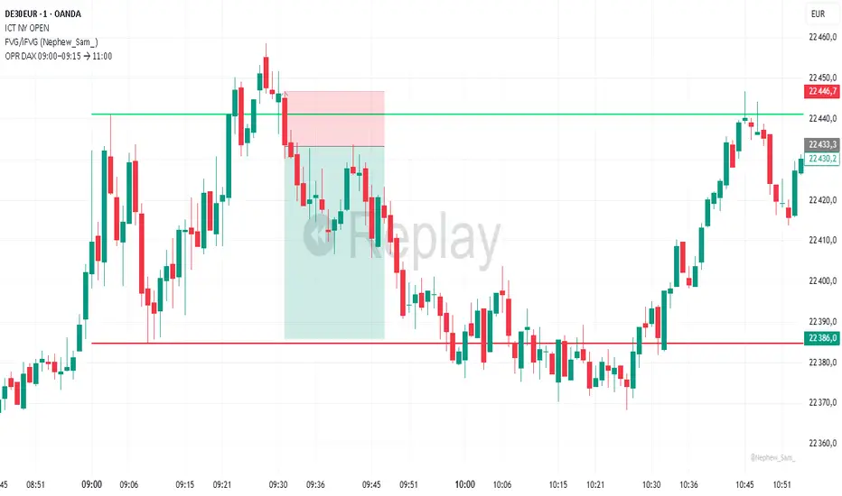
OPR DAX 09:00–09:15 → 11:00 Nico VThis indicator plots on the DAX each day:
The high (green) and low (red) of the 09:00 → 09:15 Berlin time range.
These levels are extended horizontally until 11:00.
Optionally, it displays the midpoint as a white dashed line.
Purpose: to quickly identify the morning opening range (OPR) and observe how price reacts to these levels during the rest of the morning.
Ichimoku Crypto Cloud 11-30-61A minor adjustment to the original Ichimoku Cloud, changing periods to reflect the 24/7 open market of cryptocurrency.
TENKAN: 11 - a week and a half
KIJUN: 30 - one month
SENKOU: 61 - two months
For a simpler visualization, I made the cloud limit lines and the Chikou line invisible by default.

[LunaOwl] 11 kinds of Adaptive MA Model作品: 11種自適應性平滑模型
It integrates eleven kinds of adaptive moving average method. At first, I just wanted to make a ATR. Later, the price series ±N*ATR mult, to form two series. Then use the concept of support/resistance breakthrough to design it, and then two adaptive series formation channels were formed. Take the average of the two series as the signal. When the price crosses the signal, it's judged to be long or short.
整合了十一種能夠自適應性的移動平均模型。起初只是想要做一個基本款ATR指標,後來將價格加減N個ATR倍數,形成兩條序列形成通道,再使用支撐阻力突破的概念去設計它,再形成兩條自適應性的序列形成通道,再取中間值當成信號。當價格與信號交叉,則判斷作多或者作空。
--------------------------*
Parameter 設置參數
Resolution: The default is "the same as the variety". Is a named constant for resolution input type of input function.
商品分辨率:預設與品種相同。是input函數的時間周期輸入類型的命名常量。
Smoothing: The default is Recursive Moving Average(RMA). It can choose other methods, the table is as follows.
平滑類型:預設是「遞回平均」,可以選擇其它方法,列表如下。
列表 / The table of moving averages is as follows:
//****中英對照表*****##______________________________________
1. 遞回平均 || Recursive Moving Average
2. 簡單平均 || Simple Moving Average
3. 指數平均 || Exponential Moving Average
4. 加權平均 || Weighted Moving Average
5. 船體平均 || Hull Moving Average
6. 成交量加權 || Volume Weighted Moving Average
7. 對稱加權 || Symmetric Weighted Moving Average
8. 雙重指數 || Double Exponential Moving Average
9. 三重指數 || Triple Exponential Moving Average
10. 高斯分佈 || Arnaud Legoux Moving Average
11. 提爾森T3 || Tillson T3 Moving Average
//##_________________________________________________________
Candle Mode: There are three versions, original, two-color and four-color.
燭台模式:預設模式只區分趨勢,可以改成原版蠟燭或四種顏色版本。
Length: The default is 14, usually no need to adjust.
平滑期數:預設值是14,基本上不用理它。
Occurrence: The default is 1. The range is 0~10. The larger the value, the more delayed. If zero will become too sensitive and noise.
滯後性:預設值是1。調整範圍是0~10,數值愈大信號愈延遲,如果值為0,會變得過於敏捷,那將會失去平滑的意義。
N multiple: The default is 0.618, can be set to 1. The range is 0.382~3.000.
倍數N:預設值是0.618,也可以設定1,最低是0.382,最大是3。
--------------------------*
1. Candle Mode can set the original candle, cancel candle trend color changes. However, the background will still be filled.
可以設定顯示原版的蠟燭線,背景與線並不會消失。
2. Four-color version of candles. It shows changes in trends and prices.
四色版本的蠟燭線,可以顯示趨勢與每日收盤價的變化。


ICT Killzones and Sessions W/ Silver Bullet + MacrosForex and Equity Session Tracker with Killzones, Silver Bullet, and Macro Times
This Pine Script indicator is a comprehensive timekeeping tool designed specifically for ICT traders using any time-based strategy. It helps you visualize and keep track of forex and equity session times, kill zones, macro times, and silver bullet hours.
Features:
Session and Killzone Lines:
Green: London Open (LO)
White: New York (NY)
Orange: Australian (AU)
Purple: Asian (AS)
Includes AM and PM session markers.
Dotted/Striped Lines indicate overlapping kill zones within the session timeline.
Customization Options:
Display sessions and killzones in collapsed or full view.
Hide specific sessions or killzones based on your preferences.
Customize colors, texts, and sizes.
Option to hide drawings older than the current day.
Automatic Updates:
The indicator draws all lines and boxes at the start of a new day.
Automatically adjusts time-based boxes according to the New York timezone.
Killzone Time Windows (for indices):
London KZ: 02:00 - 05:00
New York AM KZ: 07:00 - 10:00
New York PM KZ: 13:30 - 16:00
Silver Bullet Times:
03:00 - 04:00
10:00 - 11:00
14:00 - 15:00
Macro Times:
02:33 - 03:00
04:03 - 04:30
08:50 - 09:10
09:50 - 10:10
10:50 - 11:10
11:50 - 12:50
Latest Update:
January 15:
Added option to automatically change text coloring based on the chart.
Included additional optional macro times per user request:
12:50 - 13:10
13:50 - 14:15
14:50 - 15:10
15:50 - 16:15
Usage:
To maximize your experience, minimize the pane where the script is drawn. This minimizes distractions while keeping the essential time markers visible. The script is designed to help traders by clearly annotating key trading periods without overwhelming their charts.
Originality and Justification:
This indicator uniquely integrates various time-based strategies essential for ICT traders. Unlike other indicators, it consolidates session times, kill zones, macro times, and silver bullet hours into one comprehensive tool. This allows traders to have a clear and organized view of critical trading periods, facilitating better decision-making.
Credits:
This script incorporates open-source elements with significant improvements to enhance functionality and user experience.
Forex and Equity Session Tracker with Killzones, Silver Bullet, and Macro Times
This Pine Script indicator is a comprehensive timekeeping tool designed specifically for ICT traders using any time-based strategy. It helps you visualize and keep track of forex and equity session times, kill zones, macro times, and silver bullet hours.
Features:
Session and Killzone Lines:
Green: London Open (LO)
White: New York (NY)
Orange: Australian (AU)
Purple: Asian (AS)
Includes AM and PM session markers.
Dotted/Striped Lines indicate overlapping kill zones within the session timeline.
Customization Options:
Display sessions and killzones in collapsed or full view.
Hide specific sessions or killzones based on your preferences.
Customize colors, texts, and sizes.
Option to hide drawings older than the current day.
Automatic Updates:
The indicator draws all lines and boxes at the start of a new day.
Automatically adjusts time-based boxes according to the New York timezone.
Killzone Time Windows (for indices):
London KZ: 02:00 - 05:00
New York AM KZ: 07:00 - 10:00
New York PM KZ: 13:30 - 16:00
Silver Bullet Times:
03:00 - 04:00
10:00 - 11:00
14:00 - 15:00
Macro Times:
02:33 - 03:00
04:03 - 04:30
08:50 - 09:10
09:50 - 10:10
10:50 - 11:10
11:50 - 12:50
Latest Update:
January 15:
Added option to automatically change text coloring based on the chart.
Included additional optional macro times per user request:
12:50 - 13:10
13:50 - 14:15
14:50 - 15:10
15:50 - 16:15
ICT Sessions and Kill Zones
What They Are:
ICT Sessions: These are specific times during the trading day when market activity is expected to be higher, such as the London Open, New York Open, and the Asian session.
Kill Zones: These are specific time windows within these sessions where the probability of significant price movements is higher. For example, the New York AM Kill Zone is typically from 8:30 AM to 11:00 AM EST.
How to Use Them:
Identify the Session: Determine which trading session you are in (London, New York, or Asian).
Focus on Kill Zones: Within that session, focus on the kill zones for potential trade setups. For instance, during the New York session, look for setups between 8:30 AM and 11:00 AM EST.
Silver Bullets
What They Are:
Silver Bullets: These are specific, high-probability trade setups that occur within the kill zones. They are designed to be "one shot, one kill" trades, meaning they aim for precise and effective entries and exits.
How to Use Them:
Time-Based Setup: Look for these setups within the designated kill zones. For example, between 10:00 AM and 11:00 AM for the New York AM session .
Chart Analysis: Start with higher time frames like the 15-minute chart and then refine down to 5-minute and 1-minute charts to identify imbalances or specific patterns .
Macros
What They Are:
Macros: These are broader market conditions and trends that influence your trading decisions. They include understanding the overall market direction, seasonal tendencies, and the Commitment of Traders (COT) reports.
How to Use Them:
Understand Market Conditions: Be aware of the macroeconomic factors and market conditions that could affect price movements.
Seasonal Tendencies: Know the seasonal patterns that might influence the market direction.
COT Reports: Use the Commitment of Traders reports to understand the positioning of large traders and commercial hedgers .
Putting It All Together
Preparation: Understand the macro conditions and review the COT reports.
Session and Kill Zone: Identify the trading session and focus on the kill zones.
Silver Bullet Setup: Look for high-probability setups within the kill zones using refined chart analysis.
Execution: Execute the trade with precision, aiming for a "one shot, one kill" outcome.
By following these steps, you can effectively use ICT sessions, kill zones, silver bullets, and macros to enhance your trading strategy.
Usage:
To maximize your experience, shrink the pane where the script is drawn. This minimizes distractions while keeping the essential time markers visible. The script is designed to help traders by clearly annotating key trading periods without overwhelming their charts.
Originality and Justification:
This indicator uniquely integrates various time-based strategies essential for ICT traders. Unlike other indicators, it consolidates session times, kill zones, macro times, and silver bullet hours into one comprehensive tool. This allows traders to have a clear and organized view of critical trading periods, facilitating better decision-making.
Credits:
This script incorporates open-source elements with significant improvements to enhance functionality and user experience. All credit goes to itradesize for the SB + Macro boxes

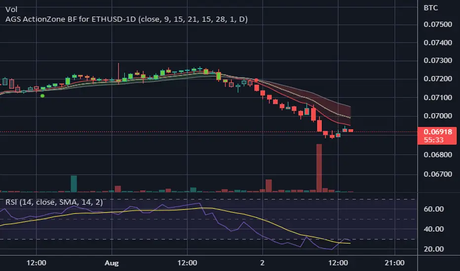
CDC ActionZone BF for ETHUSD-1D © PRoSkYNeT-EE
Based on improvements from "Kitti-Playbook Action Zone V.4.2.0.3 for Stock Market"
Based on improvements from "CDC Action Zone V3 2020 by piriya33"
Based on Triple MACD crossover between 9/15, 21/28, 15/28 for filter error signal (noise) from CDC ActionZone V3
MACDs generated from the execution of millions of times in the "Brute Force Algorithm" to backtest data from the past 5 years. ( 2017-08-21 to 2022-08-01 )
Released 2022-08-01
***** The indicator is used in the ETHUSD 1 Day period ONLY *****
Recommended Stop Loss : -4 % (execute stop Loss after candlestick has been closed)
Backtest Result ( Start $100 )
Winrate 63 % (Win:12, Loss:7, Total:19)
Live Days 1,806 days
B : Buy
S : Sell
SL : Stop Loss
2022-07-19 07 - 1,542 : B 6.971 ETH
2022-04-13 07 - 3,118 : S 8.98 % $10,750 12,7,19 63 %
2022-03-20 07 - 2,861 : B 3.448 ETH
2021-12-03 07 - 4,216 : SL -8.94 % $9,864 11,7,18 61 %
2021-11-30 07 - 4,630 : B 2.340 ETH
2021-11-18 07 - 3,997 : S 13.71 % $10,832 11,6,17 65 %
2021-10-05 07 - 3,515 : B 2.710 ETH
2021-09-20 07 - 2,977 : S 29.38 % $9,526 10,6,16 63 %
2021-07-28 07 - 2,301 : B 3.200 ETH
2021-05-20 07 - 2,769 : S 50.49 % $7,363 9,6,15 60 %
2021-03-30 07 - 1,840 : B 2.659 ETH
2021-03-22 07 - 1,681 : SL -8.29 % $4,893 8,6,14 57 %
2021-03-08 07 - 1,833 : B 2.911 ETH
2021-02-26 07 - 1,445 : S 279.27 % $5,335 8,5,13 62 %
2020-10-13 07 - 381 : B 3.692 ETH
2020-09-05 07 - 335 : S 38.43 % $1,407 7,5,12 58 %
2020-07-06 07 - 242 : B 4.199 ETH
2020-06-27 07 - 221 : S 28.49 % $1,016 6,5,11 55 %
2020-04-16 07 - 172 : B 4.598 ETH
2020-02-29 07 - 217 : S 47.62 % $791 5,5,10 50 %
2020-01-12 07 - 147 : B 3.644 ETH
2019-11-18 07 - 178 : S -2.73 % $536 4,5,9 44 %
2019-11-01 07 - 183 : B 3.010 ETH
2019-09-23 07 - 201 : SL -4.29 % $551 4,4,8 50 %
2019-09-18 07 - 210 : B 2.740 ETH
2019-07-12 07 - 275 : S 63.69 % $575 4,3,7 57 %
2019-05-03 07 - 168 : B 2.093 ETH
2019-04-28 07 - 158 : S 29.51 % $352 3,3,6 50 %
2019-02-15 07 - 122 : B 2.225 ETH
2019-01-10 07 - 125 : SL -6.02 % $271 2,3,5 40 %
2018-12-29 07 - 133 : B 2.172 ETH
2018-05-22 07 - 641 : S 5.95 % $289 2,2,4 50 %
2018-04-21 07 - 605 : B 0.451 ETH
2018-02-02 07 - 922 : S 197.42 % $273 1,2,3 33 %
2017-11-11 07 - 310 : B 0.296 ETH
2017-10-09 07 - 297 : SL -4.50 % $92 0,2,2 0 %
2017-10-07 07 - 311 : B 0.309 ETH
2017-08-22 07 - 310 : SL -4.02 % $96 0,1,1 0 %
2017-08-21 07 - 323 : B 0.310 ETH
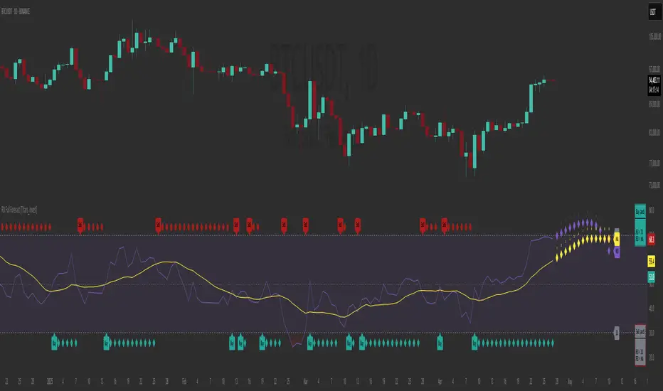
RSI Full Forecast [Titans_Invest]RSI Full Forecast
Get ready to experience the ultimate evolution of RSI-based indicators – the RSI Full Forecast, a boosted and even smarter version of the already powerful: RSI Forecast
Now featuring over 40 additional entry conditions (forecasts), this indicator redefines the way you view the market.
AI-Powered RSI Forecasting:
Using advanced linear regression with the least squares method – a solid foundation for machine learning - the RSI Full Forecast enables you to predict future RSI behavior with impressive accuracy.
But that’s not all: this new version also lets you monitor future crossovers between the RSI and the MA RSI, delivering early and strategic signals that go far beyond traditional analysis.
You’ll be able to monitor future crossovers up to 20 bars ahead, giving you an even broader and more precise view of market movements.
See the Future, Now:
• Track upcoming RSI & RSI MA crossovers in advance.
• Identify potential reversal zones before price reacts.
• Uncover statistical behavior patterns that would normally go unnoticed.
40+ Intelligent Conditions:
The new layer of conditions is designed to detect multiple high-probability scenarios based on historical patterns and predictive modeling. Each additional forecast is a window into the price's future, powered by robust mathematics and advanced algorithmic logic.
Full Customization:
All parameters can be tailored to fit your strategy – from smoothing periods to prediction sensitivity. You have complete control to turn raw data into smart decisions.
Innovative, Accurate, Unique:
This isn’t just an upgrade. It’s a quantum leap in technical analysis.
RSI Full Forecast is the first of its kind: an indicator that blends statistical analysis, machine learning, and visual design to create a true real-time predictive system.
⯁ SCIENTIFIC BASIS LINEAR REGRESSION
Linear Regression is a fundamental method of statistics and machine learning, used to model the relationship between a dependent variable y and one or more independent variables 𝑥.
The general formula for a simple linear regression is given by:
y = β₀ + β₁x + ε
β₁ = Σ((xᵢ - x̄)(yᵢ - ȳ)) / Σ((xᵢ - x̄)²)
β₀ = ȳ - β₁x̄
Where:
y = is the predicted variable (e.g. future value of RSI)
x = is the explanatory variable (e.g. time or bar index)
β0 = is the intercept (value of 𝑦 when 𝑥 = 0)
𝛽1 = is the slope of the line (rate of change)
ε = is the random error term
The goal is to estimate the coefficients 𝛽0 and 𝛽1 so as to minimize the sum of the squared errors — the so-called Random Error Method Least Squares.
⯁ LEAST SQUARES ESTIMATION
To minimize the error between predicted and observed values, we use the following formulas:
β₁ = /
β₀ = ȳ - β₁x̄
Where:
∑ = sum
x̄ = mean of x
ȳ = mean of y
x_i, y_i = individual values of the variables.
Where:
x_i and y_i are the means of the independent and dependent variables, respectively.
i ranges from 1 to n, the number of observations.
These equations guarantee the best linear unbiased estimator, according to the Gauss-Markov theorem, assuming homoscedasticity and linearity.
⯁ LINEAR REGRESSION IN MACHINE LEARNING
Linear regression is one of the cornerstones of supervised learning. Its simplicity and ability to generate accurate quantitative predictions make it essential in AI systems, predictive algorithms, time series analysis, and automated trading strategies.
By applying this model to the RSI, you are literally putting artificial intelligence at the heart of a classic indicator, bringing a new dimension to technical analysis.
⯁ VISUAL INTERPRETATION
Imagine an RSI time series like this:
Time →
RSI →
The regression line will smooth these values and extend them n periods into the future, creating a predicted trajectory based on the historical moment. This line becomes the predicted RSI, which can be crossed with the actual RSI to generate more intelligent signals.
⯁ SUMMARY OF SCIENTIFIC CONCEPTS USED
Linear Regression Models the relationship between variables using a straight line.
Least Squares Minimizes the sum of squared errors between prediction and reality.
Time Series Forecasting Estimates future values based on historical data.
Supervised Learning Trains models to predict outputs from known inputs.
Statistical Smoothing Reduces noise and reveals underlying trends.
⯁ WHY THIS INDICATOR IS REVOLUTIONARY
Scientifically-based: Based on statistical theory and mathematical inference.
Unprecedented: First public RSI with least squares predictive modeling.
Intelligent: Built with machine learning logic.
Practical: Generates forward-thinking signals.
Customizable: Flexible for any trading strategy.
⯁ CONCLUSION
By combining RSI with linear regression, this indicator allows a trader to predict market momentum, not just follow it.
RSI Full Forecast is not just an indicator — it is a scientific breakthrough in technical analysis technology.
⯁ Example of simple linear regression, which has one independent variable:
⯁ In linear regression, observations ( red ) are considered to be the result of random deviations ( green ) from an underlying relationship ( blue ) between a dependent variable ( y ) and an independent variable ( x ).
⯁ Visualizing heteroscedasticity in a scatterplot against 100 random fitted values using Matlab:
⯁ The data sets in the Anscombe's quartet are designed to have approximately the same linear regression line (as well as nearly identical means, standard deviations, and correlations) but are graphically very different. This illustrates the pitfalls of relying solely on a fitted model to understand the relationship between variables.
⯁ The result of fitting a set of data points with a quadratic function:
_________________________________________________
🔮 Linear Regression: PineScript Technical Parameters 🔮
_________________________________________________
Forecast Types:
• Flat: Assumes prices will remain the same.
• Linreg: Makes a 'Linear Regression' forecast for n periods.
Technical Information:
ta.linreg (built-in function)
Linear regression curve. A line that best fits the specified prices over a user-defined time period. It is calculated using the least squares method. The result of this function is calculated using the formula: linreg = intercept + slope * (length - 1 - offset), where intercept and slope are the values calculated using the least squares method on the source series.
Syntax:
• Function: ta.linreg()
Parameters:
• source: Source price series.
• length: Number of bars (period).
• offset: Offset.
• return: Linear regression curve.
This function has been cleverly applied to the RSI, making it capable of projecting future values based on past statistical trends.
______________________________________________________
______________________________________________________
⯁ WHAT IS THE RSI❓
The Relative Strength Index (RSI) is a technical analysis indicator developed by J. Welles Wilder. It measures the magnitude of recent price movements to evaluate overbought or oversold conditions in a market. The RSI is an oscillator that ranges from 0 to 100 and is commonly used to identify potential reversal points, as well as the strength of a trend.
⯁ HOW TO USE THE RSI❓
The RSI is calculated based on average gains and losses over a specified period (usually 14 periods). It is plotted on a scale from 0 to 100 and includes three main zones:
• Overbought: When the RSI is above 70, indicating that the asset may be overbought.
• Oversold: When the RSI is below 30, indicating that the asset may be oversold.
• Neutral Zone: Between 30 and 70, where there is no clear signal of overbought or oversold conditions.
______________________________________________________
______________________________________________________
⯁ ENTRY CONDITIONS
The conditions below are fully flexible and allow for complete customization of the signal.
______________________________________________________
______________________________________________________
🔹 CONDITIONS TO BUY 📈
______________________________________________________
• Signal Validity: The signal will remain valid for X bars .
• Signal Sequence: Configurable as AND or OR .
📈 RSI Conditions:
🔹 RSI > Upper
🔹 RSI < Upper
🔹 RSI > Lower
🔹 RSI < Lower
🔹 RSI > Middle
🔹 RSI < Middle
🔹 RSI > MA
🔹 RSI < MA
📈 MA Conditions:
🔹 MA > Upper
🔹 MA < Upper
🔹 MA > Lower
🔹 MA < Lower
📈 Crossovers:
🔹 RSI (Crossover) Upper
🔹 RSI (Crossunder) Upper
🔹 RSI (Crossover) Lower
🔹 RSI (Crossunder) Lower
🔹 RSI (Crossover) Middle
🔹 RSI (Crossunder) Middle
🔹 RSI (Crossover) MA
🔹 RSI (Crossunder) MA
🔹 MA (Crossover) Upper
🔹 MA (Crossunder) Upper
🔹 MA (Crossover) Lower
🔹 MA (Crossunder) Lower
📈 RSI Divergences:
🔹 RSI Divergence Bull
🔹 RSI Divergence Bear
📈 RSI Forecast:
🔹 RSI (Crossover) MA Forecast
🔹 RSI (Crossunder) MA Forecast
🔹 RSI Forecast 1 > MA Forecast 1
🔹 RSI Forecast 1 < MA Forecast 1
🔹 RSI Forecast 2 > MA Forecast 2
🔹 RSI Forecast 2 < MA Forecast 2
🔹 RSI Forecast 3 > MA Forecast 3
🔹 RSI Forecast 3 < MA Forecast 3
🔹 RSI Forecast 4 > MA Forecast 4
🔹 RSI Forecast 4 < MA Forecast 4
🔹 RSI Forecast 5 > MA Forecast 5
🔹 RSI Forecast 5 < MA Forecast 5
🔹 RSI Forecast 6 > MA Forecast 6
🔹 RSI Forecast 6 < MA Forecast 6
🔹 RSI Forecast 7 > MA Forecast 7
🔹 RSI Forecast 7 < MA Forecast 7
🔹 RSI Forecast 8 > MA Forecast 8
🔹 RSI Forecast 8 < MA Forecast 8
🔹 RSI Forecast 9 > MA Forecast 9
🔹 RSI Forecast 9 < MA Forecast 9
🔹 RSI Forecast 10 > MA Forecast 10
🔹 RSI Forecast 10 < MA Forecast 10
🔹 RSI Forecast 11 > MA Forecast 11
🔹 RSI Forecast 11 < MA Forecast 11
🔹 RSI Forecast 12 > MA Forecast 12
🔹 RSI Forecast 12 < MA Forecast 12
🔹 RSI Forecast 13 > MA Forecast 13
🔹 RSI Forecast 13 < MA Forecast 13
🔹 RSI Forecast 14 > MA Forecast 14
🔹 RSI Forecast 14 < MA Forecast 14
🔹 RSI Forecast 15 > MA Forecast 15
🔹 RSI Forecast 15 < MA Forecast 15
🔹 RSI Forecast 16 > MA Forecast 16
🔹 RSI Forecast 16 < MA Forecast 16
🔹 RSI Forecast 17 > MA Forecast 17
🔹 RSI Forecast 17 < MA Forecast 17
🔹 RSI Forecast 18 > MA Forecast 18
🔹 RSI Forecast 18 < MA Forecast 18
🔹 RSI Forecast 19 > MA Forecast 19
🔹 RSI Forecast 19 < MA Forecast 19
🔹 RSI Forecast 20 > MA Forecast 20
🔹 RSI Forecast 20 < MA Forecast 20
______________________________________________________
______________________________________________________
🔸 CONDITIONS TO SELL 📉
______________________________________________________
• Signal Validity: The signal will remain valid for X bars .
• Signal Sequence: Configurable as AND or OR .
📉 RSI Conditions:
🔸 RSI > Upper
🔸 RSI < Upper
🔸 RSI > Lower
🔸 RSI < Lower
🔸 RSI > Middle
🔸 RSI < Middle
🔸 RSI > MA
🔸 RSI < MA
📉 MA Conditions:
🔸 MA > Upper
🔸 MA < Upper
🔸 MA > Lower
🔸 MA < Lower
📉 Crossovers:
🔸 RSI (Crossover) Upper
🔸 RSI (Crossunder) Upper
🔸 RSI (Crossover) Lower
🔸 RSI (Crossunder) Lower
🔸 RSI (Crossover) Middle
🔸 RSI (Crossunder) Middle
🔸 RSI (Crossover) MA
🔸 RSI (Crossunder) MA
🔸 MA (Crossover) Upper
🔸 MA (Crossunder) Upper
🔸 MA (Crossover) Lower
🔸 MA (Crossunder) Lower
📉 RSI Divergences:
🔸 RSI Divergence Bull
🔸 RSI Divergence Bear
📉 RSI Forecast:
🔸 RSI (Crossover) MA Forecast
🔸 RSI (Crossunder) MA Forecast
🔸 RSI Forecast 1 > MA Forecast 1
🔸 RSI Forecast 1 < MA Forecast 1
🔸 RSI Forecast 2 > MA Forecast 2
🔸 RSI Forecast 2 < MA Forecast 2
🔸 RSI Forecast 3 > MA Forecast 3
🔸 RSI Forecast 3 < MA Forecast 3
🔸 RSI Forecast 4 > MA Forecast 4
🔸 RSI Forecast 4 < MA Forecast 4
🔸 RSI Forecast 5 > MA Forecast 5
🔸 RSI Forecast 5 < MA Forecast 5
🔸 RSI Forecast 6 > MA Forecast 6
🔸 RSI Forecast 6 < MA Forecast 6
🔸 RSI Forecast 7 > MA Forecast 7
🔸 RSI Forecast 7 < MA Forecast 7
🔸 RSI Forecast 8 > MA Forecast 8
🔸 RSI Forecast 8 < MA Forecast 8
🔸 RSI Forecast 9 > MA Forecast 9
🔸 RSI Forecast 9 < MA Forecast 9
🔸 RSI Forecast 10 > MA Forecast 10
🔸 RSI Forecast 10 < MA Forecast 10
🔸 RSI Forecast 11 > MA Forecast 11
🔸 RSI Forecast 11 < MA Forecast 11
🔸 RSI Forecast 12 > MA Forecast 12
🔸 RSI Forecast 12 < MA Forecast 12
🔸 RSI Forecast 13 > MA Forecast 13
🔸 RSI Forecast 13 < MA Forecast 13
🔸 RSI Forecast 14 > MA Forecast 14
🔸 RSI Forecast 14 < MA Forecast 14
🔸 RSI Forecast 15 > MA Forecast 15
🔸 RSI Forecast 15 < MA Forecast 15
🔸 RSI Forecast 16 > MA Forecast 16
🔸 RSI Forecast 16 < MA Forecast 16
🔸 RSI Forecast 17 > MA Forecast 17
🔸 RSI Forecast 17 < MA Forecast 17
🔸 RSI Forecast 18 > MA Forecast 18
🔸 RSI Forecast 18 < MA Forecast 18
🔸 RSI Forecast 19 > MA Forecast 19
🔸 RSI Forecast 19 < MA Forecast 19
🔸 RSI Forecast 20 > MA Forecast 20
🔸 RSI Forecast 20 < MA Forecast 20
______________________________________________________
______________________________________________________
🤖 AUTOMATION 🤖
• You can automate the BUY and SELL signals of this indicator.
______________________________________________________
______________________________________________________
⯁ UNIQUE FEATURES
______________________________________________________
Linear Regression: (Forecast)
Signal Validity: The signal will remain valid for X bars
Signal Sequence: Configurable as AND/OR
Condition Table: BUY/SELL
Condition Labels: BUY/SELL
Plot Labels in the Graph Above: BUY/SELL
Automate and Monitor Signals/Alerts: BUY/SELL
Linear Regression (Forecast)
Signal Validity: The signal will remain valid for X bars
Signal Sequence: Configurable as AND/OR
Condition Table: BUY/SELL
Condition Labels: BUY/SELL
Plot Labels in the Graph Above: BUY/SELL
Automate and Monitor Signals/Alerts: BUY/SELL
______________________________________________________
📜 SCRIPT : RSI Full Forecast
🎴 Art by : @Titans_Invest & @DiFlip
👨💻 Dev by : @Titans_Invest & @DiFlip
🎑 Titans Invest — The Wizards Without Gloves 🧤
✨ Enjoy!
______________________________________________________
o Mission 🗺
• Inspire Traders to manifest Magic in the Market.
o Vision 𐓏
• To elevate collective Energy 𐓷𐓏
PubLibCandleTrendLibrary "PubLibCandleTrend"
candle trend, multi-part candle trend, multi-part green/red candle trend, double candle trend and multi-part double candle trend conditions for indicator and strategy development
chh()
candle higher high condition
Returns: bool
chl()
candle higher low condition
Returns: bool
clh()
candle lower high condition
Returns: bool
cll()
candle lower low condition
Returns: bool
cdt()
candle double top condition
Returns: bool
cdb()
candle double bottom condition
Returns: bool
gc()
green candle condition
Returns: bool
gchh()
green candle higher high condition
Returns: bool
gchl()
green candle higher low condition
Returns: bool
gclh()
green candle lower high condition
Returns: bool
gcll()
green candle lower low condition
Returns: bool
gcdt()
green candle double top condition
Returns: bool
gcdb()
green candle double bottom condition
Returns: bool
rc()
red candle condition
Returns: bool
rchh()
red candle higher high condition
Returns: bool
rchl()
red candle higher low condition
Returns: bool
rclh()
red candle lower high condition
Returns: bool
rcll()
red candle lower low condition
Returns: bool
rcdt()
red candle double top condition
Returns: bool
rcdb()
red candle double bottom condition
Returns: bool
chh_1p()
1-part candle higher high condition
Returns: bool
chh_2p()
2-part candle higher high condition
Returns: bool
chh_3p()
3-part candle higher high condition
Returns: bool
chh_4p()
4-part candle higher high condition
Returns: bool
chh_5p()
5-part candle higher high condition
Returns: bool
chh_6p()
6-part candle higher high condition
Returns: bool
chh_7p()
7-part candle higher high condition
Returns: bool
chh_8p()
8-part candle higher high condition
Returns: bool
chh_9p()
9-part candle higher high condition
Returns: bool
chh_10p()
10-part candle higher high condition
Returns: bool
chh_11p()
11-part candle higher high condition
Returns: bool
chh_12p()
12-part candle higher high condition
Returns: bool
chh_13p()
13-part candle higher high condition
Returns: bool
chh_14p()
14-part candle higher high condition
Returns: bool
chh_15p()
15-part candle higher high condition
Returns: bool
chh_16p()
16-part candle higher high condition
Returns: bool
chh_17p()
17-part candle higher high condition
Returns: bool
chh_18p()
18-part candle higher high condition
Returns: bool
chh_19p()
19-part candle higher high condition
Returns: bool
chh_20p()
20-part candle higher high condition
Returns: bool
chh_21p()
21-part candle higher high condition
Returns: bool
chh_22p()
22-part candle higher high condition
Returns: bool
chh_23p()
23-part candle higher high condition
Returns: bool
chh_24p()
24-part candle higher high condition
Returns: bool
chh_25p()
25-part candle higher high condition
Returns: bool
chh_26p()
26-part candle higher high condition
Returns: bool
chh_27p()
27-part candle higher high condition
Returns: bool
chh_28p()
28-part candle higher high condition
Returns: bool
chh_29p()
29-part candle higher high condition
Returns: bool
chh_30p()
30-part candle higher high condition
Returns: bool
chl_1p()
1-part candle higher low condition
Returns: bool
chl_2p()
2-part candle higher low condition
Returns: bool
chl_3p()
3-part candle higher low condition
Returns: bool
chl_4p()
4-part candle higher low condition
Returns: bool
chl_5p()
5-part candle higher low condition
Returns: bool
chl_6p()
6-part candle higher low condition
Returns: bool
chl_7p()
7-part candle higher low condition
Returns: bool
chl_8p()
8-part candle higher low condition
Returns: bool
chl_9p()
9-part candle higher low condition
Returns: bool
chl_10p()
10-part candle higher low condition
Returns: bool
chl_11p()
11-part candle higher low condition
Returns: bool
chl_12p()
12-part candle higher low condition
Returns: bool
chl_13p()
13-part candle higher low condition
Returns: bool
chl_14p()
14-part candle higher low condition
Returns: bool
chl_15p()
15-part candle higher low condition
Returns: bool
chl_16p()
16-part candle higher low condition
Returns: bool
chl_17p()
17-part candle higher low condition
Returns: bool
chl_18p()
18-part candle higher low condition
Returns: bool
chl_19p()
19-part candle higher low condition
Returns: bool
chl_20p()
20-part candle higher low condition
Returns: bool
chl_21p()
21-part candle higher low condition
Returns: bool
chl_22p()
22-part candle higher low condition
Returns: bool
chl_23p()
23-part candle higher low condition
Returns: bool
chl_24p()
24-part candle higher low condition
Returns: bool
chl_25p()
25-part candle higher low condition
Returns: bool
chl_26p()
26-part candle higher low condition
Returns: bool
chl_27p()
27-part candle higher low condition
Returns: bool
chl_28p()
28-part candle higher low condition
Returns: bool
chl_29p()
29-part candle higher low condition
Returns: bool
chl_30p()
30-part candle higher low condition
Returns: bool
clh_1p()
1-part candle lower high condition
Returns: bool
clh_2p()
2-part candle lower high condition
Returns: bool
clh_3p()
3-part candle lower high condition
Returns: bool
clh_4p()
4-part candle lower high condition
Returns: bool
clh_5p()
5-part candle lower high condition
Returns: bool
clh_6p()
6-part candle lower high condition
Returns: bool
clh_7p()
7-part candle lower high condition
Returns: bool
clh_8p()
8-part candle lower high condition
Returns: bool
clh_9p()
9-part candle lower high condition
Returns: bool
clh_10p()
10-part candle lower high condition
Returns: bool
clh_11p()
11-part candle lower high condition
Returns: bool
clh_12p()
12-part candle lower high condition
Returns: bool
clh_13p()
13-part candle lower high condition
Returns: bool
clh_14p()
14-part candle lower high condition
Returns: bool
clh_15p()
15-part candle lower high condition
Returns: bool
clh_16p()
16-part candle lower high condition
Returns: bool
clh_17p()
17-part candle lower high condition
Returns: bool
clh_18p()
18-part candle lower high condition
Returns: bool
clh_19p()
19-part candle lower high condition
Returns: bool
clh_20p()
20-part candle lower high condition
Returns: bool
clh_21p()
21-part candle lower high condition
Returns: bool
clh_22p()
22-part candle lower high condition
Returns: bool
clh_23p()
23-part candle lower high condition
Returns: bool
clh_24p()
24-part candle lower high condition
Returns: bool
clh_25p()
25-part candle lower high condition
Returns: bool
clh_26p()
26-part candle lower high condition
Returns: bool
clh_27p()
27-part candle lower high condition
Returns: bool
clh_28p()
28-part candle lower high condition
Returns: bool
clh_29p()
29-part candle lower high condition
Returns: bool
clh_30p()
30-part candle lower high condition
Returns: bool
cll_1p()
1-part candle lower low condition
Returns: bool
cll_2p()
2-part candle lower low condition
Returns: bool
cll_3p()
3-part candle lower low condition
Returns: bool
cll_4p()
4-part candle lower low condition
Returns: bool
cll_5p()
5-part candle lower low condition
Returns: bool
cll_6p()
6-part candle lower low condition
Returns: bool
cll_7p()
7-part candle lower low condition
Returns: bool
cll_8p()
8-part candle lower low condition
Returns: bool
cll_9p()
9-part candle lower low condition
Returns: bool
cll_10p()
10-part candle lower low condition
Returns: bool
cll_11p()
11-part candle lower low condition
Returns: bool
cll_12p()
12-part candle lower low condition
Returns: bool
cll_13p()
13-part candle lower low condition
Returns: bool
cll_14p()
14-part candle lower low condition
Returns: bool
cll_15p()
15-part candle lower low condition
Returns: bool
cll_16p()
16-part candle lower low condition
Returns: bool
cll_17p()
17-part candle lower low condition
Returns: bool
cll_18p()
18-part candle lower low condition
Returns: bool
cll_19p()
19-part candle lower low condition
Returns: bool
cll_20p()
20-part candle lower low condition
Returns: bool
cll_21p()
21-part candle lower low condition
Returns: bool
cll_22p()
22-part candle lower low condition
Returns: bool
cll_23p()
23-part candle lower low condition
Returns: bool
cll_24p()
24-part candle lower low condition
Returns: bool
cll_25p()
25-part candle lower low condition
Returns: bool
cll_26p()
26-part candle lower low condition
Returns: bool
cll_27p()
27-part candle lower low condition
Returns: bool
cll_28p()
28-part candle lower low condition
Returns: bool
cll_29p()
29-part candle lower low condition
Returns: bool
cll_30p()
30-part candle lower low condition
Returns: bool
gc_1p()
1-part green candle condition
Returns: bool
gc_2p()
2-part green candle condition
Returns: bool
gc_3p()
3-part green candle condition
Returns: bool
gc_4p()
4-part green candle condition
Returns: bool
gc_5p()
5-part green candle condition
Returns: bool
gc_6p()
6-part green candle condition
Returns: bool
gc_7p()
7-part green candle condition
Returns: bool
gc_8p()
8-part green candle condition
Returns: bool
gc_9p()
9-part green candle condition
Returns: bool
gc_10p()
10-part green candle condition
Returns: bool
gc_11p()
11-part green candle condition
Returns: bool
gc_12p()
12-part green candle condition
Returns: bool
gc_13p()
13-part green candle condition
Returns: bool
gc_14p()
14-part green candle condition
Returns: bool
gc_15p()
15-part green candle condition
Returns: bool
gc_16p()
16-part green candle condition
Returns: bool
gc_17p()
17-part green candle condition
Returns: bool
gc_18p()
18-part green candle condition
Returns: bool
gc_19p()
19-part green candle condition
Returns: bool
gc_20p()
20-part green candle condition
Returns: bool
gc_21p()
21-part green candle condition
Returns: bool
gc_22p()
22-part green candle condition
Returns: bool
gc_23p()
23-part green candle condition
Returns: bool
gc_24p()
24-part green candle condition
Returns: bool
gc_25p()
25-part green candle condition
Returns: bool
gc_26p()
26-part green candle condition
Returns: bool
gc_27p()
27-part green candle condition
Returns: bool
gc_28p()
28-part green candle condition
Returns: bool
gc_29p()
29-part green candle condition
Returns: bool
gc_30p()
30-part green candle condition
Returns: bool
rc_1p()
1-part red candle condition
Returns: bool
rc_2p()
2-part red candle condition
Returns: bool
rc_3p()
3-part red candle condition
Returns: bool
rc_4p()
4-part red candle condition
Returns: bool
rc_5p()
5-part red candle condition
Returns: bool
rc_6p()
6-part red candle condition
Returns: bool
rc_7p()
7-part red candle condition
Returns: bool
rc_8p()
8-part red candle condition
Returns: bool
rc_9p()
9-part red candle condition
Returns: bool
rc_10p()
10-part red candle condition
Returns: bool
rc_11p()
11-part red candle condition
Returns: bool
rc_12p()
12-part red candle condition
Returns: bool
rc_13p()
13-part red candle condition
Returns: bool
rc_14p()
14-part red candle condition
Returns: bool
rc_15p()
15-part red candle condition
Returns: bool
rc_16p()
16-part red candle condition
Returns: bool
rc_17p()
17-part red candle condition
Returns: bool
rc_18p()
18-part red candle condition
Returns: bool
rc_19p()
19-part red candle condition
Returns: bool
rc_20p()
20-part red candle condition
Returns: bool
rc_21p()
21-part red candle condition
Returns: bool
rc_22p()
22-part red candle condition
Returns: bool
rc_23p()
23-part red candle condition
Returns: bool
rc_24p()
24-part red candle condition
Returns: bool
rc_25p()
25-part red candle condition
Returns: bool
rc_26p()
26-part red candle condition
Returns: bool
rc_27p()
27-part red candle condition
Returns: bool
rc_28p()
28-part red candle condition
Returns: bool
rc_29p()
29-part red candle condition
Returns: bool
rc_30p()
30-part red candle condition
Returns: bool
cdut()
candle double uptrend condition
Returns: bool
cddt()
candle double downtrend condition
Returns: bool
cdut_1p()
1-part candle double uptrend condition
Returns: bool
cdut_2p()
2-part candle double uptrend condition
Returns: bool
cdut_3p()
3-part candle double uptrend condition
Returns: bool
cdut_4p()
4-part candle double uptrend condition
Returns: bool
cdut_5p()
5-part candle double uptrend condition
Returns: bool
cdut_6p()
6-part candle double uptrend condition
Returns: bool
cdut_7p()
7-part candle double uptrend condition
Returns: bool
cdut_8p()
8-part candle double uptrend condition
Returns: bool
cdut_9p()
9-part candle double uptrend condition
Returns: bool
cdut_10p()
10-part candle double uptrend condition
Returns: bool
cdut_11p()
11-part candle double uptrend condition
Returns: bool
cdut_12p()
12-part candle double uptrend condition
Returns: bool
cdut_13p()
13-part candle double uptrend condition
Returns: bool
cdut_14p()
14-part candle double uptrend condition
Returns: bool
cdut_15p()
15-part candle double uptrend condition
Returns: bool
cdut_16p()
16-part candle double uptrend condition
Returns: bool
cdut_17p()
17-part candle double uptrend condition
Returns: bool
cdut_18p()
18-part candle double uptrend condition
Returns: bool
cdut_19p()
19-part candle double uptrend condition
Returns: bool
cdut_20p()
20-part candle double uptrend condition
Returns: bool
cdut_21p()
21-part candle double uptrend condition
Returns: bool
cdut_22p()
22-part candle double uptrend condition
Returns: bool
cdut_23p()
23-part candle double uptrend condition
Returns: bool
cdut_24p()
24-part candle double uptrend condition
Returns: bool
cdut_25p()
25-part candle double uptrend condition
Returns: bool
cdut_26p()
26-part candle double uptrend condition
Returns: bool
cdut_27p()
27-part candle double uptrend condition
Returns: bool
cdut_28p()
28-part candle double uptrend condition
Returns: bool
cdut_29p()
29-part candle double uptrend condition
Returns: bool
cdut_30p()
30-part candle double uptrend condition
Returns: bool
cddt_1p()
1-part candle double downtrend condition
Returns: bool
cddt_2p()
2-part candle double downtrend condition
Returns: bool
cddt_3p()
3-part candle double downtrend condition
Returns: bool
cddt_4p()
4-part candle double downtrend condition
Returns: bool
cddt_5p()
5-part candle double downtrend condition
Returns: bool
cddt_6p()
6-part candle double downtrend condition
Returns: bool
cddt_7p()
7-part candle double downtrend condition
Returns: bool
cddt_8p()
8-part candle double downtrend condition
Returns: bool
cddt_9p()
9-part candle double downtrend condition
Returns: bool
cddt_10p()
10-part candle double downtrend condition
Returns: bool
cddt_11p()
11-part candle double downtrend condition
Returns: bool
cddt_12p()
12-part candle double downtrend condition
Returns: bool
cddt_13p()
13-part candle double downtrend condition
Returns: bool
cddt_14p()
14-part candle double downtrend condition
Returns: bool
cddt_15p()
15-part candle double downtrend condition
Returns: bool
cddt_16p()
16-part candle double downtrend condition
Returns: bool
cddt_17p()
17-part candle double downtrend condition
Returns: bool
cddt_18p()
18-part candle double downtrend condition
Returns: bool
cddt_19p()
19-part candle double downtrend condition
Returns: bool
cddt_20p()
20-part candle double downtrend condition
Returns: bool
cddt_21p()
21-part candle double downtrend condition
Returns: bool
cddt_22p()
22-part candle double downtrend condition
Returns: bool
cddt_23p()
23-part candle double downtrend condition
Returns: bool
cddt_24p()
24-part candle double downtrend condition
Returns: bool
cddt_25p()
25-part candle double downtrend condition
Returns: bool
cddt_26p()
26-part candle double downtrend condition
Returns: bool
cddt_27p()
27-part candle double downtrend condition
Returns: bool
cddt_28p()
28-part candle double downtrend condition
Returns: bool
cddt_29p()
29-part candle double downtrend condition
Returns: bool
cddt_30p()
30-part candle double downtrend condition
Returns: bool
Drip's 11am rule breakout/breakdown (OG)This indicator is based on Drippy2hard's 11:30 am (EST) rule.
In simple terms the rule states that:
If a trending stock makes a new high after 11:15-11:30am EST, there is a 75% chance of closing within 1% of High of day (HOD). Same applies for downtrend.
Please note:
Not all stocks will abide by this, this is backtested on stocks with avg daily volume > 2M and mostly mega cap stocks which have liquid option chains. The backtesting results show very promising results on $SPY/ $SPX so it is advised to trade $SPY/ $SPX using this indicator over any other stocks.
Although the name suggests 11 AM rule, the backtesting shows higher win rate for 11:30 AM so please select that option in the settings.
As always, no indicator is perfect and please follow your risk management and understand that indicators are tools to aid your trading and by no means they are supposed to work as intended in all scenarios
How the script works
1. A HOD/LOD zone is identified based on regular session (9:30am-11:30am) EST. Users can select cut off time to 11AM in the settings. These will be indicated on chart after 11/11:30pm depending on what user selected
2. If the stock breaks above the HOD and the ADX is showing strong momentum to upside then the candlesticks will start showing neon color, if the trend based on moving averages and candle closing is also bullish then the indicator will show trend arrows under the candle indicating to stay in the trade. Same applies for break below LOD, only the colors will change to represent downtrend.
3. An optional cloud is also shown if the trend is developed. The cloud can be used as trail stop or re entry point as long as it is displayed on chart
How to use the indicator in trading
In general, there are three scenarios which are trade worthy
1. If the stocks breaks out above the HOD zone and up trend develops or the stocks breaks below the LOD zone and downtrend develops. See images below
2. You can also use the LOD/HOD zone as demand/ supply if the Price action is range bound like this example below
Thanks for reading, please give thumbs up if you like using it! Please post comments on how to use it.

[astropark] Power Tools Overlay//******************************************************************************
// Power Tools Overlay
// Inner Version 1.2.1 13/12/2018
// Developer: iDelphi
// Developer: astropark (Ichimoku Cloud), SMA EMA & Cross tools
//------------------------------------------------------------------------------
// 21/11/2018 Added EMA SMA WMA
// 21/11/2018 Added SMA-EMA EMA-WMA WMA-SMA (Thanks to mariobros1 for the idea of the Simultaneous MA)
// 21/11/2018 Added Bollinger Bands
// 21/11/2018 Added Ichimoku Cloud (Thanks to astropark for all the code of the Ichimoku Cloud)
// 23/11/2018 Show all the indicator as default
// 23/11/2018 Added a cross when single Moving Averages crossing (Thanks to astropark for the idea)
// 24/11/2018 Descriptions Fix
// 24/11/2018 Added Option to enable/disable all Moving Averages
// 10/12/2018 Added EMAs and Crosses
// 13/12/2018 indicator number fixes
//******************************************************************************

[astropark] Power Tools Overlay//******************************************************************************
// Power Tools Overlay
// Inner Version 1.2 20/12/2018
// Developer: iDelphi
// Developer: astropark (Ichimoku Cloud), SMA EMA & Cross tools
//------------------------------------------------------------------------------
// 21/11/2018 Added EMA SMA WMA
// 21/11/2018 Added SMA-EMA EMA-WMA WMA-SMA (Thanks to mariobros1 for the idea of the Simultaneous MA)
// 21/11/2018 Added Bollinger Bands
// 21/11/2018 Added Ichimoku Cloud (Thanks to astropark for all the code of the Ichimoku Cloud)
// 23/11/2018 Show all the indicator as default
// 23/11/2018 Added a cross when single Moving Averages crossing (Thanks to astropark for the idea)
// 24/11/2018 Descriptions Fix
// 24/11/2018 Added Option to enable/disable all Moving Averages
// 10/12/2018 Added EMAs and Crosses
//******************************************************************************

ADR% Extension Levels from SMA 50I created this indicator inspired by RealSimpleAriel (a swing trader I recommend following on X) who does not buy stocks extended beyond 4 ADR% from the 50 SMA and uses extensions from the 50 SMA at 7-8-9-10-11-12-13 ADR% to take profits with a 20% position trimming.
RealSimpleAriel's strategy (as I understood it):
-> Focuses on leading stocks from leading groups and industries, i.e., those that have grown the most in the last 1-3-6 months (see on Finviz groups and then select sector-industry).
-> Targets stocks with the best technical setup for a breakout, above the 200 SMA in a bear market and above both the 50 SMA and 200 SMA in a bull market, selecting those with growing Earnings and Sales.
-> Buys stocks on breakout with a stop loss set at the day's low of the breakout and ensures they are not extended beyond 4 ADR% from the 50 SMA.
-> 3-5 day momentum burst: After a breakout, takes profits by selling 1/2 or 1/3 of the position after a 3-5 day upward move.
-> 20% trimming on extension from the 50 SMA: At 7 ADR% (ADR% calculated over 20 days) extension from the 50 SMA, takes profits by selling 20% of the remaining position. Continues to trim 20% of the remaining position based on the stock price extension from the 50 SMA, calculated using the 20-period ADR%, thus trimming 20% at 8-9-10-11 ADR% extension from the 50 SMA. Upon reaching 12-13 ADR% extension from the 50 SMA, considers the stock overextended, closes the remaining position, and evaluates a short.
-> Trailing stop with ascending SMA: Uses a chosen SMA (10, 20, or 50) as the definitive stop loss for the position, depending on the stock's movement speed (preferring larger SMAs for slower-moving stocks or for long-term theses). If the stock's closing price falls below the chosen SMA, the entire position is closed.
In summary:
-->Buy a breakout using the day's low of the breakout as the stop loss (this stop loss is the most critical).
--> Do not buy stocks extended beyond 4 ADR% from the 50 SMA.
--> Sell 1/2 or 1/3 of the position after 3-5 days of upward movement.
--> Trim 20% of the position at each 7-8-9-10-11-12-13 ADR% extension from the 50 SMA.
--> Close the entire position if the breakout fails and the day's low of the breakout is reached.
--> Close the entire position if the price, during the rise, falls below a chosen SMA (10, 20, or 50, depending on your preference).
--> Definitively close the position if it reaches 12-13 ADR% extension from the 50 SMA.
I used Grok from X to create this indicator. I am not a programmer, but based on the ADR% I use, it works.
Below is Grok from X's description of the indicator:
Script Description
The script is a custom indicator for TradingView that displays extension levels based on ADR% relative to the 50-period Simple Moving Average (SMA). Below is a detailed description of its features, structure, and behavior:
1. Purpose of the Indicator
Name: "ADR% Extension Levels from SMA 50".
Objective: Draw horizontal blue lines above and below the 50-period SMA, corresponding to specific ADR% multiples (4, 7, 8, 9, 10, 11, 12, 13). These levels represent potential price extension zones based on the average daily percentage volatility.
Overlay: The indicator is overlaid on the price chart (overlay=true), so the lines and SMA appear directly on the price graph.
2. Configurable Inputs
The indicator allows users to customize parameters through TradingView settings:
SMA Length (smaLength):
Default: 50 periods.
Description: Specifies the number of periods for calculating the Simple Moving Average (SMA). The 50-period SMA serves as the reference point for extension levels.
Constraint: Minimum 1 period.
ADR% Length (adrLength):
Default: 20 periods.
Description: Specifies the number of days to calculate the moving average of the daily high/low ratio, used to determine ADR%.
Constraint: Minimum 1 period.
Scale Factor (scaleFactor):
Default: 1.0.
Description: An optional multiplier to adjust the distance of extension levels from the SMA. Useful if levels are too close or too far due to an overly small or large ADR%.
Constraint: Minimum 0.1, increments of 0.1.
Tooltip: "Adjust if levels are too close or far from SMA".
3. Main Calculations
50-period SMA:
Calculated with ta.sma(close, smaLength) using the closing price (close).
Serves as the central line around which extension levels are drawn.
ADR% (Average Daily Range Percentage):
Formula: 100 * (ta.sma(dhigh / dlow, adrLength) - 1).
Details:
dhigh and dlow are the daily high and low prices, obtained via request.security(syminfo.tickerid, "D", high/low) to ensure data is daily-based, regardless of the chart's timeframe.
The dhigh / dlow ratio represents the daily percentage change.
The simple moving average (ta.sma) of this ratio over 20 days (adrLength) is subtracted by 1 and multiplied by 100 to obtain ADR% as a percentage.
The result is multiplied by scaleFactor for manual adjustments.
Extension Levels:
Defined as ADR% multiples: 4, 7, 8, 9, 10, 11, 12, 13.
Stored in an array (levels) for easy iteration.
For each level, prices above and below the SMA are calculated as:
Above: sma50 * (1 + (level * adrPercent / 100))
Below: sma50 * (1 - (level * adrPercent / 100))
These represent price levels corresponding to a percentage change from the SMA equal to level * ADR%.
4. Visualization
Horizontal Blue Lines:
For each level (4, 7, 8, 9, 10, 11, 12, 13 ADR%), two lines are drawn:
One above the SMA (e.g., +4 ADR%).
One below the SMA (e.g., -4 ADR%).
Color: Blue (color.blue).
Style: Solid (style=line.style_solid).
Management:
Each level has dedicated variables for upper and lower lines (e.g., upperLine1, lowerLine1 for 4 ADR%).
Previous lines are deleted with line.delete before drawing new ones to avoid overlaps.
Lines are updated at each bar with line.new(bar_index , level, bar_index, level), covering the range from the previous bar to the current one.
Labels:
Displayed only on the last bar (barstate.islast) to avoid clutter.
For each level, two labels:
Above: E.g., "4 ADR%", positioned above the upper line (style=label.style_label_down).
Below: E.g., "-4 ADR%", positioned below the lower line (style=label.style_label_up).
Color: Blue background, white text.
50-period SMA:
Drawn as a gray line (color.gray) for visual reference.
Diagnostics:
ADR% Plot: ADR% is plotted in the status line (orange, histogram style) to verify the value.
ADR% Label: A label on the last bar near the SMA shows the exact ADR% value (e.g., "ADR%: 2.34%"), with a gray background and white text.
5. Behavior
Dynamic Updating:
Lines update with each new bar to reflect new SMA 50 and ADR% values.
Since ADR% uses daily data ("D"), it remains constant within the same day but changes day-to-day.
Visibility Across All Bars:
Lines are drawn on every bar, not just the last one, ensuring visibility on historical data as well.
Adaptability:
The scaleFactor allows level adjustments if ADR% is too small (e.g., for low-volatility symbols) or too large (e.g., for cryptocurrencies).
Compatibility:
Works on any timeframe since ADR% is calculated from daily data.
Suitable for symbols with varying volatility (e.g., stocks, forex, cryptocurrencies).
6. Intended Use
Technical Analysis: Extension levels represent significant price zones based on average daily volatility. They can be used to:
Identify potential price targets (e.g., take profit at +7 ADR%).
Assess support/resistance zones (e.g., -4 ADR% as support).
Measure price extension relative to the 50 SMA.
Trading: Useful for strategies based on breakouts or mean reversion, where ADR% levels indicate reversal or continuation points.
Debugging: Labels and ADR% plot help verify that values align with the symbol’s volatility.
7. Limitations
Dependence on Daily Data: ADR% is based on daily dhigh/dlow, so it may not reflect intraday volatility on short timeframes (e.g., 1 minute).
Extreme ADR% Values: For low-volatility symbols (e.g., bonds) or high-volatility symbols (e.g., meme stocks), ADR% may require adjustments via scaleFactor.
Graphical Load: Drawing 16 lines (8 upper, 8 lower) on every bar may slow the chart for very long historical periods, though line management is optimized.
ADR% Formula: The formula 100 * (sma(dhigh/dlow, Length) - 1) may produce different values compared to other ADR% definitions (e.g., (high - low) / close * 100), so users should be aware of the context.
8. Visual Example
On a chart of a stock like TSLA (daily timeframe):
The 50 SMA is a gray line tracking the average trend.
Assuming an ADR% of 3%:
At +4 ADR% (12%), a blue line appears at sma50 * 1.12.
At -4 ADR% (-12%), a blue line appears at sma50 * 0.88.
Other lines appear at ±7, ±8, ±9, ±10, ±11, ±12, ±13 ADR%.
On the last bar, labels show "4 ADR%", "-4 ADR%", etc., and a gray label shows "ADR%: 3.00%".
ADR% is visible in the status line as an orange histogram.
9. Code: Technical Structure
Language: Pine Script @version=5.
Inputs: Three configurable parameters (smaLength, adrLength, scaleFactor).
Calculations:
SMA: ta.sma(close, smaLength).
ADR%: 100 * (ta.sma(dhigh / dlow, adrLength) - 1) * scaleFactor.
Levels: sma50 * (1 ± (level * adrPercent / 100)).
Graphics:
Lines: Created with line.new, deleted with line.delete to avoid overlaps.
Labels: Created with label.new only on the last bar.
Plots: plot(sma50) for the SMA, plot(adrPercent) for debugging.
Optimization: Uses dedicated variables for each line (e.g., upperLine1, lowerLine1) for clear management and to respect TradingView’s graphical object limits.
10. Possible Improvements
Option to show lines only on the last bar: Would reduce visual clutter.
Customizable line styles: Allow users to choose color or style (e.g., dashed).
Alert for anomalous ADR%: A message if ADR% is too small or large.
Dynamic levels: Allow users to specify ADR% multiples via input.
Optimization for short timeframes: Adapt ADR% for intraday timeframes.
Conclusion
The script creates a visual indicator that helps traders identify price extension levels based on daily volatility (ADR%) relative to the 50 SMA. It is robust, configurable, and includes debugging tools (ADR% plot and labels) to verify values. The ADR% formula based on dhigh/dlow

STD/C-Filtered, N-Order Power-of-Cosine FIR Filter [Loxx]STD/C-Filtered, N-Order Power-of-Cosine FIR Filter is a Discrete-Time, FIR Digital Filter that uses Power-of-Cosine Family of FIR filters. This is an N-order algorithm that turns the following indicator from a static max 16 orders to a N orders, but limited to 50 in code. You can change the top end value if you with to higher orders than 50, but the signal is likely too noisy at that level. This indicator also includes a clutter and standard deviation filter.
See the static order version of this indicator here:
STD/C-Filtered, Power-of-Cosine FIR Filter
Amplitudes for STD/C-Filtered, N-Order Power-of-Cosine FIR Filter:
What are FIR Filters?
In discrete-time signal processing, windowing is a preliminary signal shaping technique, usually applied to improve the appearance and usefulness of a subsequent Discrete Fourier Transform. Several window functions can be defined, based on a constant (rectangular window), B-splines, other polynomials, sinusoids, cosine-sums, adjustable, hybrid, and other types. The windowing operation consists of multipying the given sampled signal by the window function. For trading purposes, these FIR filters act as advanced weighted moving averages.
What is Power-of-Sine Digital FIR Filter?
Also called Cos^alpha Window Family. In this family of windows, changing the value of the parameter alpha generates different windows.
f(n) = math.cos(alpha) * (math.pi * n / N) , 0 ≤ |n| ≤ N/2
where alpha takes on integer values and N is a even number
General expanded form:
alpha0 - alpha1 * math.cos(2 * math.pi * n / N)
+ alpha2 * math.cos(4 * math.pi * n / N)
- alpha3 * math.cos(4 * math.pi * n / N)
+ alpha4 * math.cos(6 * math.pi * n / N)
- ...
Special Cases for alpha:
alpha = 0: Rectangular window, this is also just the SMA (not included here)
alpha = 1: MLT sine window (not included here)
alpha = 2: Hann window (raised cosine = cos^2)
alpha = 4: Alternative Blackman (maximized roll-off rate)
This indicator contains a binomial expansion algorithm to handle N orders of a cosine power series. You can read about how this is done here: The Binomial Theorem
What is Pascal's Triangle and how was it used here?
In mathematics, Pascal's triangle is a triangular array of the binomial coefficients that arises in probability theory, combinatorics, and algebra. In much of the Western world, it is named after the French mathematician Blaise Pascal, although other mathematicians studied it centuries before him in India, Persia, China, Germany, and Italy.
The rows of Pascal's triangle are conventionally enumerated starting with row n = 0 at the top (the 0th row). The entries in each row are numbered from the left beginning with k=0 and are usually staggered relative to the numbers in the adjacent rows. The triangle may be constructed in the following manner: In row 0 (the topmost row), there is a unique nonzero entry 1. Each entry of each subsequent row is constructed by adding the number above and to the left with the number above and to the right, treating blank entries as 0. For example, the initial number in the first (or any other) row is 1 (the sum of 0 and 1), whereas the numbers 1 and 3 in the third row are added to produce the number 4 in the fourth row.
Rows of Pascal's Triangle
0 Order: 1
1 Order: 1 1
2 Order: 1 2 1
3 Order: 1 3 3 1
4 Order: 1 4 6 4 1
5 Order: 1 5 10 10 5 1
6 Order: 1 6 15 20 15 6 1
7 Order: 1 7 21 35 35 21 7 1
8 Order: 1 8 28 56 70 56 28 8 1
9 Order: 1 9 36 34 84 126 126 84 36 9 1
10 Order: 1 10 45 120 210 252 210 120 45 10 1
11 Order: 1 11 55 165 330 462 462 330 165 55 11 1
12 Order: 1 12 66 220 495 792 924 792 495 220 66 12 1
13 Order: 1 13 78 286 715 1287 1716 1716 1287 715 286 78 13 1
For a 12th order Power-of-Cosine FIR Filter
1. We take the coefficients from the Left side of the 12th row
1 13 78 286 715 1287 1716 1716 1287 715 286 78 13 1
2. We slice those in half to
1 13 78 286 715 1287 1716
3. We reverse the array
1716 1287 715 286 78 13 1
This is our array of alphas: alpha1, alpha2, ... alphaN
4. We then pull alpha one from the previous order, order 11, the middle value
11 Order: 1 11 55 165 330 462 462 330 165 55 11 1
The middle value is 462, this value becomes our alpha0 in the calculation
5. We apply these alphas to the cosine calculations
example: + alpha4 * math.cos(6 * math.pi * n / N)
6. We then divide by the sum of the alphas to derive our final coefficient weighting kernel
**This is only useful for orders that are EVEN, if you use odd ordering, the following are the coefficient outputs and these aren't useful since they cancel each other out and result in a value of zero. See below for an odd numbered oder and compare with the amplitude of the graphic posted above of the even order amplitude:
What is a Standard Deviation Filter?
If price or output or both don't move more than the (standard deviation) * multiplier then the trend stays the previous bar trend. This will appear on the chart as "stepping" of the moving average line. This works similar to Super Trend or Parabolic SAR but is a more naive technique of filtering.
What is a Clutter Filter?
For our purposes here, this is a filter that compares the slope of the trading filter output to a threshold to determine whether to shift trends. If the slope is up but the slope doesn't exceed the threshold, then the color is gray and this indicates a chop zone. If the slope is down but the slope doesn't exceed the threshold, then the color is gray and this indicates a chop zone. Alternatively if either up or down slope exceeds the threshold then the trend turns green for up and red for down. Fro demonstration purposes, an EMA is used as the moving average. This acts to reduce the noise in the signal.
Included
Bar coloring
Loxx's Expanded Source Types
Signals
Alerts

BTC and ETH Long strategy - version 2I wrote my first article in May 2020. See below
BTC and ETH Long strategy - version1
After 6 months, it is now time to check the result of my script for the last 6 months.
XBTUSD (4H): 14/05/2020 --> 22/11/2020 = +78% in 4 trades
ETHXBT (4H): 14/05/2020 --> 22/11/2020 = +21% in 9 trades
ETHUSD (4H): 14/05/2020 --> 22/11/2020 = +90% in 6 trades
Using the signals from this strategy to trade manually has shown that this was a bit frustrating because of the low rate of winning trades.
If you have to enter 100 trades and see 75% of them failing and 25% winning, this is frustrating. For sure the strategy makes good money but it is difficult to hold this mentality.
So, I have reviewed and modified it to get a higher winning rate.
After few days of work, tests and validation, I managed to get a wining rate close to 60%.
The key element was also to decrease the number of trades by using a higher time frame. (4H candles instead of 2H candles).
- Entry in position is based on
MACD, EMA (20), SMA (100), SMA (200) moving up
AND EMA (20) > SMA (100)
AND SMA (100) > SMA (200)
- Exit the position if: Stoploss is reached OR EMA (20) crossUnder SMA (100)
The goal of this new script is to be able to follow the signals manually and only make few trades per years.
I have also validated it against some other altcoins where some are giving very good results.
Here are some results for 2020 (from 01/01/2020 until now (22/11/2020). Those results are the one I get when using 4H candles.
ETH/USD: +144% in 8 trades.
BTC/USD: +120% in 7 trades.
ETH/BTC: +33% in 9 trades.
ICX/USD: +123% in 10 trades.
LINK/USD: +155% in 11 trades.
MLN/USD: +388% in 8 trades.
ADA/USD: +180% in 7 trades.
LINK/BTC: +97% in 10 trades.
The best is that above results are without considering compound effect. If you re-invest all gains done in each new trade, this will give you the below results :)
ETH/USD: +189% in 8 trades.
BTC/USD: +260% in 7 trades.
ETH/BTC: +29% in 9 trades.
ICX/USD: +112% in 10 trades.
LINK/USD: +222% in 11 trades.
MLN/USD: +793% in 8 trades.
ADA/USD: +319% in 7 trades.
LINK/BTC: +103% in 10 trades.
As you can see, the results are good and the number of trades for 11 months is not big, which allows the trader to place orders manually.
But still, I'm lazy :), so, I have also coded this strategy in HaasScript language which allows you to automate this strategy using the HaasOnline software specialized in automated crypto trading.
I hope that this strategy will give you ideas or will be the starting point for your own strategy.
Let me know if you need more details.
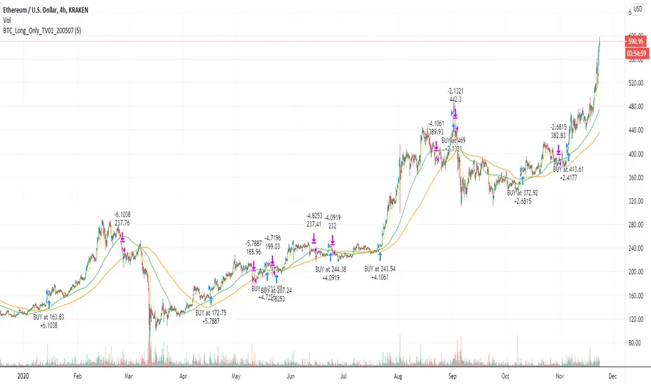
Drummond Geometry - Pldot and EnvelopeThis Pine Script will:
1.Calculate and display the PL Dot (Price Level Dot), a moving average that reflects short-term market trends.
2.Plot the Envelope Top and Bottom lines based on averages of previous highs and lows, which represent key areas of resistance and support.
Drummond Geometry Overview
Drummond Geometry is a method of market analysis focused on:
PL Dot : Captures market energy and trend direction. It reacts to price deviations and serves as a magnet for price returns, often referred to as a "PL Dot Refresh."
Envelope Theory : Considers price movements as cycles oscillating between the Envelope Top and Bottom. Prices breaking these boundaries often indicate trends, retracements, or exhaustion.
The geometry helps traders visualize energy flows in the market and anticipate directional changes using established support and resistance zones.
Understanding PL Dot and Envelope Top/Bottom
PL Dot:
Formula: Average(Average(H, L, C) of last three bars)
Usage: Indicates short-term trends:
Trend: PL Dot slopes upward or downward.
Congestion: PL Dot moves horizontally.
Envelope Top and Bottom:
Formula:
Top: (11 H1 + 11 H2 + 11 H3) / 3
Bottom: (11 L1 + 11 L2 + 11 L3) / 3
Usage: Acts as dynamic resistance and support:
Price above the top: Indicates strong bullish momentum.
Price below the bottom: Indicates strong bearish momentum.
Advantages of Drummond Geometry
Clarity of Market Flow: Highlights the relationship between price and key levels (PL Dot, Envelope Top/Bottom).
Predictive Power: Suggests possible reversals or continuation based on energy distribution.
Adaptability: Works across multiple time frames and market types (trending, congestion).
Trading Strategy
PL Dot Trades:
Buy: When price returns to the PL Dot in an uptrend.
Sell: When price returns to the PL Dot in a downtrend.
Envelope Trades:
Reversal: Trade counter to price if it breaks and retreats from the Envelope Top/Bottom.
Continuation: Trade in the direction of price if it sustains movement beyond the Envelope Top/Bottom.

LV Stock QualityCritical financial and technical values are listed in the table.
PIOTROSKI_F_SCORE (expect. >5) -> The Piotroski score is a discrete score between zero and nine that reflects nine criteria used to determine the strength of a firm's financial position. The Piotroski score is used to determine the best value stocks, with nine being the best and zero being the worst. Having a score bigger than 5 is a good sign for the strength of a firm's financial position
ROE (expect. >11) --> Return on equity (ROE) is a measure of a company's financial performance. It is calculated by dividing net income by shareholders' equity. Because shareholders' equity is equal to a company’s assets minus its debt, ROE is a way of showing a company's return on net assets. A “good” ROE will depend on the company’s industry and competitors.
EPS_GROWTH (expect. >11) --> This indicator is calculated as the percentage change in Basic earnings per share for one year. This indicator reflects the growth rate of a company's basic profit per share outstanding for one year. It is calculated based using only common shares. An increase in EPS growth may signal that a company is becoming more profitable and efficient in its operations. A decline in EPS growth may signal that a company is spending more or losing business share. EPS growth should be viewed alongside other metrics like revenue and costs.
CURRENT_RATIO (expect. >1.25) --> The current ratio measures a company’s ability to pay current, or short-term, liabilities (debt and payables) with its current, or short-term, assets (cash, inventory, and receivables). Current ratios over 1.00 indicate that a company's current assets are greater than its current liabilities, meaning it could more easily pay of short-term debts.
OPERATING_MARGIN(expect. >11) --> The operating margin measures how much profit a company makes on a dollar of sales after paying for variable costs of production, such as wages and raw materials, but before paying interest or tax.
RETURN_CAPITAL (expect. >11) --> Return of capital (ROC) is a payment that an investor receives as a portion of their original investment and that is not considered income or capital gains from the investment.
ALTMAN_Z_SCORE (expect. >1.8) --> The Altman Z-score is the output of a credit-strength test that gauges a publicly traded manufacturing company's likelihood of bankruptcy. An Altman Z-score close to 0 suggests a company might be headed for bankruptcy, while a score closer to 3 suggests a company is in solid financial positioning.
REVENUE_GROWTH (expect. >11) --> Quarterly revenue growth is an increase in a company's sales in one quarter compared to sales of a different quarter. Comparing a company's financials from one period to another gives a clear picture of its revenue growth rate and can help investors identify the catalyst for such growth.
SUSTAINABLE_GROWTH (expect. >11) --> The sustainable growth rate (SGR) is the maximum rate of growth that a company or social enterprise can sustain without having to finance growth with additional equity or debt. In other words, it is the rate at which the company can grow while using its own internal revenue without borrowing from outside sources.
DEBT TO INCOME (expect. <0.4) --> A debt-to-income (DTI) ratio is a financial metric used by lenders to determine your borrowing risk. Your DTI ratio represents the total amount of debt you owe compared to the total amount of money you earn each month.
NORMALIZED ATR (expect. <8, W) --> The Normalized Average True Range (Normalized ATR) is an indicator used to measure market volatility by normalizing the average true range values. It does this by dividing the Average True Range (ATR) by the asset's closing price, converting it into a percentage. This normalization allows for the comparison of volatility levels across different securities or market conditions, regardless of the asset's price levels. The Normalized ATR helps traders to adjust their strategies based on relative volatility, rather than absolute price movements.
INDEX expect. EMA10>EMA20 --> it is expected to have EMA 10 > EMA 20 in weekly basis graph. It is known that having a strong trend in index will also increases chance of strong trend on stock levels. You need to select INDEX Market of stock via settings.
M. RELATIVE STRENGTH expect. MRS>1 --> Stan Weinstein uses the Mansfield RS indicator as another relative strength indicator. The indicator measures the variation in the 52-week ratio of stock and market.
VOLUME CHANGE (expect. >30) --> Having an increase on volume comparing to previous week can be a good sign if it occurs at the same time of breakout.
PRICE CHANGE (expect. >5 and <20) --> Having an increase on price comparing to previous week can be a good sign if it occurs at the same time of breakout.
It is better to look on weekly basis graphs.
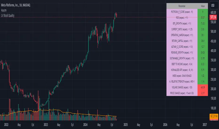
PubLibTrendLibrary "PubLibTrend"
trend, multi-part trend, double trend and multi-part double trend conditions for indicator and strategy development
rlut()
return line uptrend condition
Returns: bool
dt()
downtrend condition
Returns: bool
ut()
uptrend condition
Returns: bool
rldt()
return line downtrend condition
Returns: bool
dtop()
double top condition
Returns: bool
dbot()
double bottom condition
Returns: bool
rlut_1p()
1-part return line uptrend condition
Returns: bool
rlut_2p()
2-part return line uptrend condition
Returns: bool
rlut_3p()
3-part return line uptrend condition
Returns: bool
rlut_4p()
4-part return line uptrend condition
Returns: bool
rlut_5p()
5-part return line uptrend condition
Returns: bool
rlut_6p()
6-part return line uptrend condition
Returns: bool
rlut_7p()
7-part return line uptrend condition
Returns: bool
rlut_8p()
8-part return line uptrend condition
Returns: bool
rlut_9p()
9-part return line uptrend condition
Returns: bool
rlut_10p()
10-part return line uptrend condition
Returns: bool
rlut_11p()
11-part return line uptrend condition
Returns: bool
rlut_12p()
12-part return line uptrend condition
Returns: bool
rlut_13p()
13-part return line uptrend condition
Returns: bool
rlut_14p()
14-part return line uptrend condition
Returns: bool
rlut_15p()
15-part return line uptrend condition
Returns: bool
rlut_16p()
16-part return line uptrend condition
Returns: bool
rlut_17p()
17-part return line uptrend condition
Returns: bool
rlut_18p()
18-part return line uptrend condition
Returns: bool
rlut_19p()
19-part return line uptrend condition
Returns: bool
rlut_20p()
20-part return line uptrend condition
Returns: bool
rlut_21p()
21-part return line uptrend condition
Returns: bool
rlut_22p()
22-part return line uptrend condition
Returns: bool
rlut_23p()
23-part return line uptrend condition
Returns: bool
rlut_24p()
24-part return line uptrend condition
Returns: bool
rlut_25p()
25-part return line uptrend condition
Returns: bool
rlut_26p()
26-part return line uptrend condition
Returns: bool
rlut_27p()
27-part return line uptrend condition
Returns: bool
rlut_28p()
28-part return line uptrend condition
Returns: bool
rlut_29p()
29-part return line uptrend condition
Returns: bool
rlut_30p()
30-part return line uptrend condition
Returns: bool
dt_1p()
1-part downtrend condition
Returns: bool
dt_2p()
2-part downtrend condition
Returns: bool
dt_3p()
3-part downtrend condition
Returns: bool
dt_4p()
4-part downtrend condition
Returns: bool
dt_5p()
5-part downtrend condition
Returns: bool
dt_6p()
6-part downtrend condition
Returns: bool
dt_7p()
7-part downtrend condition
Returns: bool
dt_8p()
8-part downtrend condition
Returns: bool
dt_9p()
9-part downtrend condition
Returns: bool
dt_10p()
10-part downtrend condition
Returns: bool
dt_11p()
11-part downtrend condition
Returns: bool
dt_12p()
12-part downtrend condition
Returns: bool
dt_13p()
13-part downtrend condition
Returns: bool
dt_14p()
14-part downtrend condition
Returns: bool
dt_15p()
15-part downtrend condition
Returns: bool
dt_16p()
16-part downtrend condition
Returns: bool
dt_17p()
17-part downtrend condition
Returns: bool
dt_18p()
18-part downtrend condition
Returns: bool
dt_19p()
19-part downtrend condition
Returns: bool
dt_20p()
20-part downtrend condition
Returns: bool
dt_21p()
21-part downtrend condition
Returns: bool
dt_22p()
22-part downtrend condition
Returns: bool
dt_23p()
23-part downtrend condition
Returns: bool
dt_24p()
24-part downtrend condition
Returns: bool
dt_25p()
25-part downtrend condition
Returns: bool
dt_26p()
26-part downtrend condition
Returns: bool
dt_27p()
27-part downtrend condition
Returns: bool
dt_28p()
28-part downtrend condition
Returns: bool
dt_29p()
29-part downtrend condition
Returns: bool
dt_30p()
30-part downtrend condition
Returns: bool
ut_1p()
1-part uptrend condition
Returns: bool
ut_2p()
2-part uptrend condition
Returns: bool
ut_3p()
3-part uptrend condition
Returns: bool
ut_4p()
4-part uptrend condition
Returns: bool
ut_5p()
5-part uptrend condition
Returns: bool
ut_6p()
6-part uptrend condition
Returns: bool
ut_7p()
7-part uptrend condition
Returns: bool
ut_8p()
8-part uptrend condition
Returns: bool
ut_9p()
9-part uptrend condition
Returns: bool
ut_10p()
10-part uptrend condition
Returns: bool
ut_11p()
11-part uptrend condition
Returns: bool
ut_12p()
12-part uptrend condition
Returns: bool
ut_13p()
13-part uptrend condition
Returns: bool
ut_14p()
14-part uptrend condition
Returns: bool
ut_15p()
15-part uptrend condition
Returns: bool
ut_16p()
16-part uptrend condition
Returns: bool
ut_17p()
17-part uptrend condition
Returns: bool
ut_18p()
18-part uptrend condition
Returns: bool
ut_19p()
19-part uptrend condition
Returns: bool
ut_20p()
20-part uptrend condition
Returns: bool
ut_21p()
21-part uptrend condition
Returns: bool
ut_22p()
22-part uptrend condition
Returns: bool
ut_23p()
23-part uptrend condition
Returns: bool
ut_24p()
24-part uptrend condition
Returns: bool
ut_25p()
25-part uptrend condition
Returns: bool
ut_26p()
26-part uptrend condition
Returns: bool
ut_27p()
27-part uptrend condition
Returns: bool
ut_28p()
28-part uptrend condition
Returns: bool
ut_29p()
29-part uptrend condition
Returns: bool
ut_30p()
30-part uptrend condition
Returns: bool
rldt_1p()
1-part return line downtrend condition
Returns: bool
rldt_2p()
2-part return line downtrend condition
Returns: bool
rldt_3p()
3-part return line downtrend condition
Returns: bool
rldt_4p()
4-part return line downtrend condition
Returns: bool
rldt_5p()
5-part return line downtrend condition
Returns: bool
rldt_6p()
6-part return line downtrend condition
Returns: bool
rldt_7p()
7-part return line downtrend condition
Returns: bool
rldt_8p()
8-part return line downtrend condition
Returns: bool
rldt_9p()
9-part return line downtrend condition
Returns: bool
rldt_10p()
10-part return line downtrend condition
Returns: bool
rldt_11p()
11-part return line downtrend condition
Returns: bool
rldt_12p()
12-part return line downtrend condition
Returns: bool
rldt_13p()
13-part return line downtrend condition
Returns: bool
rldt_14p()
14-part return line downtrend condition
Returns: bool
rldt_15p()
15-part return line downtrend condition
Returns: bool
rldt_16p()
16-part return line downtrend condition
Returns: bool
rldt_17p()
17-part return line downtrend condition
Returns: bool
rldt_18p()
18-part return line downtrend condition
Returns: bool
rldt_19p()
19-part return line downtrend condition
Returns: bool
rldt_20p()
20-part return line downtrend condition
Returns: bool
rldt_21p()
21-part return line downtrend condition
Returns: bool
rldt_22p()
22-part return line downtrend condition
Returns: bool
rldt_23p()
23-part return line downtrend condition
Returns: bool
rldt_24p()
24-part return line downtrend condition
Returns: bool
rldt_25p()
25-part return line downtrend condition
Returns: bool
rldt_26p()
26-part return line downtrend condition
Returns: bool
rldt_27p()
27-part return line downtrend condition
Returns: bool
rldt_28p()
28-part return line downtrend condition
Returns: bool
rldt_29p()
29-part return line downtrend condition
Returns: bool
rldt_30p()
30-part return line downtrend condition
Returns: bool
dut()
double uptrend condition
Returns: bool
ddt()
double downtrend condition
Returns: bool
dut_1p()
1-part double uptrend condition
Returns: bool
dut_2p()
2-part double uptrend condition
Returns: bool
dut_3p()
3-part double uptrend condition
Returns: bool
dut_4p()
4-part double uptrend condition
Returns: bool
dut_5p()
5-part double uptrend condition
Returns: bool
dut_6p()
6-part double uptrend condition
Returns: bool
dut_7p()
7-part double uptrend condition
Returns: bool
dut_8p()
8-part double uptrend condition
Returns: bool
dut_9p()
9-part double uptrend condition
Returns: bool
dut_10p()
10-part double uptrend condition
Returns: bool
dut_11p()
11-part double uptrend condition
Returns: bool
dut_12p()
12-part double uptrend condition
Returns: bool
dut_13p()
13-part double uptrend condition
Returns: bool
dut_14p()
14-part double uptrend condition
Returns: bool
dut_15p()
15-part double uptrend condition
Returns: bool
dut_16p()
16-part double uptrend condition
Returns: bool
dut_17p()
17-part double uptrend condition
Returns: bool
dut_18p()
18-part double uptrend condition
Returns: bool
dut_19p()
19-part double uptrend condition
Returns: bool
dut_20p()
20-part double uptrend condition
Returns: bool
dut_21p()
21-part double uptrend condition
Returns: bool
dut_22p()
22-part double uptrend condition
Returns: bool
dut_23p()
23-part double uptrend condition
Returns: bool
dut_24p()
24-part double uptrend condition
Returns: bool
dut_25p()
25-part double uptrend condition
Returns: bool
dut_26p()
26-part double uptrend condition
Returns: bool
dut_27p()
27-part double uptrend condition
Returns: bool
dut_28p()
28-part double uptrend condition
Returns: bool
dut_29p()
29-part double uptrend condition
Returns: bool
dut_30p()
30-part double uptrend condition
Returns: bool
ddt_1p()
1-part double downtrend condition
Returns: bool
ddt_2p()
2-part double downtrend condition
Returns: bool
ddt_3p()
3-part double downtrend condition
Returns: bool
ddt_4p()
4-part double downtrend condition
Returns: bool
ddt_5p()
5-part double downtrend condition
Returns: bool
ddt_6p()
6-part double downtrend condition
Returns: bool
ddt_7p()
7-part double downtrend condition
Returns: bool
ddt_8p()
8-part double downtrend condition
Returns: bool
ddt_9p()
9-part double downtrend condition
Returns: bool
ddt_10p()
10-part double downtrend condition
Returns: bool
ddt_11p()
11-part double downtrend condition
Returns: bool
ddt_12p()
12-part double downtrend condition
Returns: bool
ddt_13p()
13-part double downtrend condition
Returns: bool
ddt_14p()
14-part double downtrend condition
Returns: bool
ddt_15p()
15-part double downtrend condition
Returns: bool
ddt_16p()
16-part double downtrend condition
Returns: bool
ddt_17p()
17-part double downtrend condition
Returns: bool
ddt_18p()
18-part double downtrend condition
Returns: bool
ddt_19p()
19-part double downtrend condition
Returns: bool
ddt_20p()
20-part double downtrend condition
Returns: bool
ddt_21p()
21-part double downtrend condition
Returns: bool
ddt_22p()
22-part double downtrend condition
Returns: bool
ddt_23p()
23-part double downtrend condition
Returns: bool
ddt_24p()
24-part double downtrend condition
Returns: bool
ddt_25p()
25-part double downtrend condition
Returns: bool
ddt_26p()
26-part double downtrend condition
Returns: bool
ddt_27p()
27-part double downtrend condition
Returns: bool
ddt_28p()
28-part double downtrend condition
Returns: bool
ddt_29p()
29-part double downtrend condition
Returns: bool
ddt_30p()
30-part double downtrend condition
Returns: bool

Sladkaya BulochkaAccording to the statistics of Thomas Bulkovski collected over several years on the 1-minute chart (21 million candles), there is a statistically significant periods, where the higher the probability of reversal rates on short-term timeframe.
By reversal, on average, had in mind the movement to 5 candles.
This three periods, they remain unchanged, depending on the hour:
- the first minute of each hour (10:01, 11:01, etc.)
- the first minute after the hour (10:31, 11:31)
- 51 minutes each hour (10:51, 11:51)
------------------------------------------------------
По статистике Томаса Булковски, собранной за несколько лет на 1-минутном графике (21 миллион свечей), есть статистически значимые периоды, где более высока вероятность разворота цены на краткосрочных ТФ.
Под разворотом, в среднем, имелось в виду движение на 5 свечей.
Это три периода, они неизменны в зависимости от часа:
- первая минута каждого часа (10:01, 11:01 и т.д.)
- первая минута после получаса (10:31, 11:31)
- каждая 51 минута часа (10:51, 11:51)
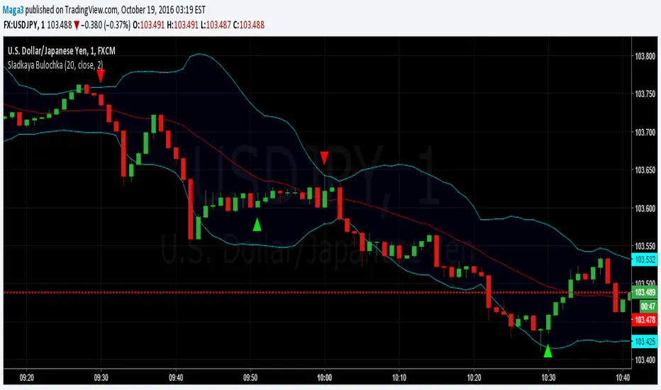
Markov Chain [3D] | FractalystWhat exactly is a Markov Chain?
This indicator uses a Markov Chain model to analyze, quantify, and visualize the transitions between market regimes (Bull, Bear, Neutral) on your chart. It dynamically detects these regimes in real-time, calculates transition probabilities, and displays them as animated 3D spheres and arrows, giving traders intuitive insight into current and future market conditions.
How does a Markov Chain work, and how should I read this spheres-and-arrows diagram?
Think of three weather modes: Sunny, Rainy, Cloudy.
Each sphere is one mode. The loop on a sphere means “stay the same next step” (e.g., Sunny again tomorrow).
The arrows leaving a sphere show where things usually go next if they change (e.g., Sunny moving to Cloudy).
Some paths matter more than others. A more prominent loop means the current mode tends to persist. A more prominent outgoing arrow means a change to that destination is the usual next step.
Direction isn’t symmetric: moving Sunny→Cloudy can behave differently than Cloudy→Sunny.
Now relabel the spheres to markets: Bull, Bear, Neutral.
Spheres: market regimes (uptrend, downtrend, range).
Self‑loop: tendency for the current regime to continue on the next bar.
Arrows: the most common next regime if a switch happens.
How to read: Start at the sphere that matches current bar state. If the loop stands out, expect continuation. If one outgoing path stands out, that switch is the typical next step. Opposite directions can differ (Bear→Neutral doesn’t have to match Neutral→Bear).
What states and transitions are shown?
The three market states visualized are:
Bullish (Bull): Upward or strong-market regime.
Bearish (Bear): Downward or weak-market regime.
Neutral: Sideways or range-bound regime.
Bidirectional animated arrows and probability labels show how likely the market is to move from one regime to another (e.g., Bull → Bear or Neutral → Bull).
How does the regime detection system work?
You can use either built-in price returns (based on adaptive Z-score normalization) or supply three custom indicators (such as volume, oscillators, etc.).
Values are statistically normalized (Z-scored) over a configurable lookback period.
The normalized outputs are classified into Bull, Bear, or Neutral zones.
If using three indicators, their regime signals are averaged and smoothed for robustness.
How are transition probabilities calculated?
On every confirmed bar, the algorithm tracks the sequence of detected market states, then builds a rolling window of transitions.
The code maintains a transition count matrix for all regime pairs (e.g., Bull → Bear).
Transition probabilities are extracted for each possible state change using Laplace smoothing for numerical stability, and frequently updated in real-time.
What is unique about the visualization?
3D animated spheres represent each regime and change visually when active.
Animated, bidirectional arrows reveal transition probabilities and allow you to see both dominant and less likely regime flows.
Particles (moving dots) animate along the arrows, enhancing the perception of regime flow direction and speed.
All elements dynamically update with each new price bar, providing a live market map in an intuitive, engaging format.
Can I use custom indicators for regime classification?
Yes! Enable the "Custom Indicators" switch and select any three chart series as inputs. These will be normalized and combined (each with equal weight), broadening the regime classification beyond just price-based movement.
What does the “Lookback Period” control?
Lookback Period (default: 100) sets how much historical data builds the probability matrix. Shorter periods adapt faster to regime changes but may be noisier. Longer periods are more stable but slower to adapt.
How is this different from a Hidden Markov Model (HMM)?
It sets the window for both regime detection and probability calculations. Lower values make the system more reactive, but potentially noisier. Higher values smooth estimates and make the system more robust.
How is this Markov Chain different from a Hidden Markov Model (HMM)?
Markov Chain (as here): All market regimes (Bull, Bear, Neutral) are directly observable on the chart. The transition matrix is built from actual detected regimes, keeping the model simple and interpretable.
Hidden Markov Model: The actual regimes are unobservable ("hidden") and must be inferred from market output or indicator "emissions" using statistical learning algorithms. HMMs are more complex, can capture more subtle structure, but are harder to visualize and require additional machine learning steps for training.
A standard Markov Chain models transitions between observable states using a simple transition matrix, while a Hidden Markov Model assumes the true states are hidden (latent) and must be inferred from observable “emissions” like price or volume data. In practical terms, a Markov Chain is transparent and easier to implement and interpret; an HMM is more expressive but requires statistical inference to estimate hidden states from data.
Markov Chain: states are observable; you directly count or estimate transition probabilities between visible states. This makes it simpler, faster, and easier to validate and tune.
HMM: states are hidden; you only observe emissions generated by those latent states. Learning involves machine learning/statistical algorithms (commonly Baum–Welch/EM for training and Viterbi for decoding) to infer both the transition dynamics and the most likely hidden state sequence from data.
How does the indicator avoid “repainting” or look-ahead bias?
All regime changes and matrix updates happen only on confirmed (closed) bars, so no future data is leaked, ensuring reliable real-time operation.
Are there practical tuning tips?
Tune the Lookback Period for your asset/timeframe: shorter for fast markets, longer for stability.
Use custom indicators if your asset has unique regime drivers.
Watch for rapid changes in transition probabilities as early warning of a possible regime shift.
Who is this indicator for?
Quants and quantitative researchers exploring probabilistic market modeling, especially those interested in regime-switching dynamics and Markov models.
Programmers and system developers who need a probabilistic regime filter for systematic and algorithmic backtesting:
The Markov Chain indicator is ideally suited for programmatic integration via its bias output (1 = Bull, 0 = Neutral, -1 = Bear).
Although the visualization is engaging, the core output is designed for automated, rules-based workflows—not for discretionary/manual trading decisions.
Developers can connect the indicator’s output directly to their Pine Script logic (using input.source()), allowing rapid and robust backtesting of regime-based strategies.
It acts as a plug-and-play regime filter: simply plug the bias output into your entry/exit logic, and you have a scientifically robust, probabilistically-derived signal for filtering, timing, position sizing, or risk regimes.
The MC's output is intentionally "trinary" (1/0/-1), focusing on clear regime states for unambiguous decision-making in code. If you require nuanced, multi-probability or soft-label state vectors, consider expanding the indicator or stacking it with a probability-weighted logic layer in your scripting.
Because it avoids subjectivity, this approach is optimal for systematic quants, algo developers building backtested, repeatable strategies based on probabilistic regime analysis.
What's the mathematical foundation behind this?
The mathematical foundation behind this Markov Chain indicator—and probabilistic regime detection in finance—draws from two principal models: the (standard) Markov Chain and the Hidden Markov Model (HMM).
How to use this indicator programmatically?
The Markov Chain indicator automatically exports a bias value (+1 for Bullish, -1 for Bearish, 0 for Neutral) as a plot visible in the Data Window. This allows you to integrate its regime signal into your own scripts and strategies for backtesting, automation, or live trading.
Step-by-Step Integration with Pine Script (input.source)
Add the Markov Chain indicator to your chart.
This must be done first, since your custom script will "pull" the bias signal from the indicator's plot.
In your strategy, create an input using input.source()
Example:
//@version=5
strategy("MC Bias Strategy Example")
mcBias = input.source(close, "MC Bias Source")
After saving, go to your script’s settings. For the “MC Bias Source” input, select the plot/output of the Markov Chain indicator (typically its bias plot).
Use the bias in your trading logic
Example (long only on Bull, flat otherwise):
if mcBias == 1
strategy.entry("Long", strategy.long)
else
strategy.close("Long")
For more advanced workflows, combine mcBias with additional filters or trailing stops.
How does this work behind-the-scenes?
TradingView’s input.source() lets you use any plot from another indicator as a real-time, “live” data feed in your own script (source).
The selected bias signal is available to your Pine code as a variable, enabling logical decisions based on regime (trend-following, mean-reversion, etc.).
This enables powerful strategy modularity : decouple regime detection from entry/exit logic, allowing fast experimentation without rewriting core signal code.
Integrating 45+ Indicators with Your Markov Chain — How & Why
The Enhanced Custom Indicators Export script exports a massive suite of over 45 technical indicators—ranging from classic momentum (RSI, MACD, Stochastic, etc.) to trend, volume, volatility, and oscillator tools—all pre-calculated, centered/scaled, and available as plots.
// Enhanced Custom Indicators Export - 45 Technical Indicators
// Comprehensive technical analysis suite for advanced market regime detection
//@version=6
indicator('Enhanced Custom Indicators Export | Fractalyst', shorttitle='Enhanced CI Export', overlay=false, scale=scale.right, max_labels_count=500, max_lines_count=500)
// |----- Input Parameters -----| //
momentum_group = "Momentum Indicators"
trend_group = "Trend Indicators"
volume_group = "Volume Indicators"
volatility_group = "Volatility Indicators"
oscillator_group = "Oscillator Indicators"
display_group = "Display Settings"
// Common lengths
length_14 = input.int(14, "Standard Length (14)", minval=1, maxval=100, group=momentum_group)
length_20 = input.int(20, "Medium Length (20)", minval=1, maxval=200, group=trend_group)
length_50 = input.int(50, "Long Length (50)", minval=1, maxval=200, group=trend_group)
// Display options
show_table = input.bool(true, "Show Values Table", group=display_group)
table_size = input.string("Small", "Table Size", options= , group=display_group)
// |----- MOMENTUM INDICATORS (15 indicators) -----| //
// 1. RSI (Relative Strength Index)
rsi_14 = ta.rsi(close, length_14)
rsi_centered = rsi_14 - 50
// 2. Stochastic Oscillator
stoch_k = ta.stoch(close, high, low, length_14)
stoch_d = ta.sma(stoch_k, 3)
stoch_centered = stoch_k - 50
// 3. Williams %R
williams_r = ta.stoch(close, high, low, length_14) - 100
// 4. MACD (Moving Average Convergence Divergence)
= ta.macd(close, 12, 26, 9)
// 5. Momentum (Rate of Change)
momentum = ta.mom(close, length_14)
momentum_pct = (momentum / close ) * 100
// 6. Rate of Change (ROC)
roc = ta.roc(close, length_14)
// 7. Commodity Channel Index (CCI)
cci = ta.cci(close, length_20)
// 8. Money Flow Index (MFI)
mfi = ta.mfi(close, length_14)
mfi_centered = mfi - 50
// 9. Awesome Oscillator (AO)
ao = ta.sma(hl2, 5) - ta.sma(hl2, 34)
// 10. Accelerator Oscillator (AC)
ac = ao - ta.sma(ao, 5)
// 11. Chande Momentum Oscillator (CMO)
cmo = ta.cmo(close, length_14)
// 12. Detrended Price Oscillator (DPO)
dpo = close - ta.sma(close, length_20)
// 13. Price Oscillator (PPO)
ppo = ta.sma(close, 12) - ta.sma(close, 26)
ppo_pct = (ppo / ta.sma(close, 26)) * 100
// 14. TRIX
trix_ema1 = ta.ema(close, length_14)
trix_ema2 = ta.ema(trix_ema1, length_14)
trix_ema3 = ta.ema(trix_ema2, length_14)
trix = ta.roc(trix_ema3, 1) * 10000
// 15. Klinger Oscillator
klinger = ta.ema(volume * (high + low + close) / 3, 34) - ta.ema(volume * (high + low + close) / 3, 55)
// 16. Fisher Transform
fisher_hl2 = 0.5 * (hl2 - ta.lowest(hl2, 10)) / (ta.highest(hl2, 10) - ta.lowest(hl2, 10)) - 0.25
fisher = 0.5 * math.log((1 + fisher_hl2) / (1 - fisher_hl2))
// 17. Stochastic RSI
stoch_rsi = ta.stoch(rsi_14, rsi_14, rsi_14, length_14)
stoch_rsi_centered = stoch_rsi - 50
// 18. Relative Vigor Index (RVI)
rvi_num = ta.swma(close - open)
rvi_den = ta.swma(high - low)
rvi = rvi_den != 0 ? rvi_num / rvi_den : 0
// 19. Balance of Power (BOP)
bop = (close - open) / (high - low)
// |----- TREND INDICATORS (10 indicators) -----| //
// 20. Simple Moving Average Momentum
sma_20 = ta.sma(close, length_20)
sma_momentum = ((close - sma_20) / sma_20) * 100
// 21. Exponential Moving Average Momentum
ema_20 = ta.ema(close, length_20)
ema_momentum = ((close - ema_20) / ema_20) * 100
// 22. Parabolic SAR
sar = ta.sar(0.02, 0.02, 0.2)
sar_trend = close > sar ? 1 : -1
// 23. Linear Regression Slope
lr_slope = ta.linreg(close, length_20, 0) - ta.linreg(close, length_20, 1)
// 24. Moving Average Convergence (MAC)
mac = ta.sma(close, 10) - ta.sma(close, 30)
// 25. Trend Intensity Index (TII)
tii_sum = 0.0
for i = 1 to length_20
tii_sum += close > close ? 1 : 0
tii = (tii_sum / length_20) * 100
// 26. Ichimoku Cloud Components
ichimoku_tenkan = (ta.highest(high, 9) + ta.lowest(low, 9)) / 2
ichimoku_kijun = (ta.highest(high, 26) + ta.lowest(low, 26)) / 2
ichimoku_signal = ichimoku_tenkan > ichimoku_kijun ? 1 : -1
// 27. MESA Adaptive Moving Average (MAMA)
mama_alpha = 2.0 / (length_20 + 1)
mama = ta.ema(close, length_20)
mama_momentum = ((close - mama) / mama) * 100
// 28. Zero Lag Exponential Moving Average (ZLEMA)
zlema_lag = math.round((length_20 - 1) / 2)
zlema_data = close + (close - close )
zlema = ta.ema(zlema_data, length_20)
zlema_momentum = ((close - zlema) / zlema) * 100
// |----- VOLUME INDICATORS (6 indicators) -----| //
// 29. On-Balance Volume (OBV)
obv = ta.obv
// 30. Volume Rate of Change (VROC)
vroc = ta.roc(volume, length_14)
// 31. Price Volume Trend (PVT)
pvt = ta.pvt
// 32. Negative Volume Index (NVI)
nvi = 0.0
nvi := volume < volume ? nvi + ((close - close ) / close ) * nvi : nvi
// 33. Positive Volume Index (PVI)
pvi = 0.0
pvi := volume > volume ? pvi + ((close - close ) / close ) * pvi : pvi
// 34. Volume Oscillator
vol_osc = ta.sma(volume, 5) - ta.sma(volume, 10)
// 35. Ease of Movement (EOM)
eom_distance = high - low
eom_box_height = volume / 1000000
eom = eom_box_height != 0 ? eom_distance / eom_box_height : 0
eom_sma = ta.sma(eom, length_14)
// 36. Force Index
force_index = volume * (close - close )
force_index_sma = ta.sma(force_index, length_14)
// |----- VOLATILITY INDICATORS (10 indicators) -----| //
// 37. Average True Range (ATR)
atr = ta.atr(length_14)
atr_pct = (atr / close) * 100
// 38. Bollinger Bands Position
bb_basis = ta.sma(close, length_20)
bb_dev = 2.0 * ta.stdev(close, length_20)
bb_upper = bb_basis + bb_dev
bb_lower = bb_basis - bb_dev
bb_position = bb_dev != 0 ? (close - bb_basis) / bb_dev : 0
bb_width = bb_dev != 0 ? (bb_upper - bb_lower) / bb_basis * 100 : 0
// 39. Keltner Channels Position
kc_basis = ta.ema(close, length_20)
kc_range = ta.ema(ta.tr, length_20)
kc_upper = kc_basis + (2.0 * kc_range)
kc_lower = kc_basis - (2.0 * kc_range)
kc_position = kc_range != 0 ? (close - kc_basis) / kc_range : 0
// 40. Donchian Channels Position
dc_upper = ta.highest(high, length_20)
dc_lower = ta.lowest(low, length_20)
dc_basis = (dc_upper + dc_lower) / 2
dc_position = (dc_upper - dc_lower) != 0 ? (close - dc_basis) / (dc_upper - dc_lower) : 0
// 41. Standard Deviation
std_dev = ta.stdev(close, length_20)
std_dev_pct = (std_dev / close) * 100
// 42. Relative Volatility Index (RVI)
rvi_up = ta.stdev(close > close ? close : 0, length_14)
rvi_down = ta.stdev(close < close ? close : 0, length_14)
rvi_total = rvi_up + rvi_down
rvi_volatility = rvi_total != 0 ? (rvi_up / rvi_total) * 100 : 50
// 43. Historical Volatility
hv_returns = math.log(close / close )
hv = ta.stdev(hv_returns, length_20) * math.sqrt(252) * 100
// 44. Garman-Klass Volatility
gk_vol = math.log(high/low) * math.log(high/low) - (2*math.log(2)-1) * math.log(close/open) * math.log(close/open)
gk_volatility = math.sqrt(ta.sma(gk_vol, length_20)) * 100
// 45. Parkinson Volatility
park_vol = math.log(high/low) * math.log(high/low)
parkinson = math.sqrt(ta.sma(park_vol, length_20) / (4 * math.log(2))) * 100
// 46. Rogers-Satchell Volatility
rs_vol = math.log(high/close) * math.log(high/open) + math.log(low/close) * math.log(low/open)
rogers_satchell = math.sqrt(ta.sma(rs_vol, length_20)) * 100
// |----- OSCILLATOR INDICATORS (5 indicators) -----| //
// 47. Elder Ray Index
elder_bull = high - ta.ema(close, 13)
elder_bear = low - ta.ema(close, 13)
elder_power = elder_bull + elder_bear
// 48. Schaff Trend Cycle (STC)
stc_macd = ta.ema(close, 23) - ta.ema(close, 50)
stc_k = ta.stoch(stc_macd, stc_macd, stc_macd, 10)
stc_d = ta.ema(stc_k, 3)
stc = ta.stoch(stc_d, stc_d, stc_d, 10)
// 49. Coppock Curve
coppock_roc1 = ta.roc(close, 14)
coppock_roc2 = ta.roc(close, 11)
coppock = ta.wma(coppock_roc1 + coppock_roc2, 10)
// 50. Know Sure Thing (KST)
kst_roc1 = ta.roc(close, 10)
kst_roc2 = ta.roc(close, 15)
kst_roc3 = ta.roc(close, 20)
kst_roc4 = ta.roc(close, 30)
kst = ta.sma(kst_roc1, 10) + 2*ta.sma(kst_roc2, 10) + 3*ta.sma(kst_roc3, 10) + 4*ta.sma(kst_roc4, 15)
// 51. Percentage Price Oscillator (PPO)
ppo_line = ((ta.ema(close, 12) - ta.ema(close, 26)) / ta.ema(close, 26)) * 100
ppo_signal = ta.ema(ppo_line, 9)
ppo_histogram = ppo_line - ppo_signal
// |----- PLOT MAIN INDICATORS -----| //
// Plot key momentum indicators
plot(rsi_centered, title="01_RSI_Centered", color=color.purple, linewidth=1)
plot(stoch_centered, title="02_Stoch_Centered", color=color.blue, linewidth=1)
plot(williams_r, title="03_Williams_R", color=color.red, linewidth=1)
plot(macd_histogram, title="04_MACD_Histogram", color=color.orange, linewidth=1)
plot(cci, title="05_CCI", color=color.green, linewidth=1)
// Plot trend indicators
plot(sma_momentum, title="06_SMA_Momentum", color=color.navy, linewidth=1)
plot(ema_momentum, title="07_EMA_Momentum", color=color.maroon, linewidth=1)
plot(sar_trend, title="08_SAR_Trend", color=color.teal, linewidth=1)
plot(lr_slope, title="09_LR_Slope", color=color.lime, linewidth=1)
plot(mac, title="10_MAC", color=color.fuchsia, linewidth=1)
// Plot volatility indicators
plot(atr_pct, title="11_ATR_Pct", color=color.yellow, linewidth=1)
plot(bb_position, title="12_BB_Position", color=color.aqua, linewidth=1)
plot(kc_position, title="13_KC_Position", color=color.olive, linewidth=1)
plot(std_dev_pct, title="14_StdDev_Pct", color=color.silver, linewidth=1)
plot(bb_width, title="15_BB_Width", color=color.gray, linewidth=1)
// Plot volume indicators
plot(vroc, title="16_VROC", color=color.blue, linewidth=1)
plot(eom_sma, title="17_EOM", color=color.red, linewidth=1)
plot(vol_osc, title="18_Vol_Osc", color=color.green, linewidth=1)
plot(force_index_sma, title="19_Force_Index", color=color.orange, linewidth=1)
plot(obv, title="20_OBV", color=color.purple, linewidth=1)
// Plot additional oscillators
plot(ao, title="21_Awesome_Osc", color=color.navy, linewidth=1)
plot(cmo, title="22_CMO", color=color.maroon, linewidth=1)
plot(dpo, title="23_DPO", color=color.teal, linewidth=1)
plot(trix, title="24_TRIX", color=color.lime, linewidth=1)
plot(fisher, title="25_Fisher", color=color.fuchsia, linewidth=1)
// Plot more momentum indicators
plot(mfi_centered, title="26_MFI_Centered", color=color.yellow, linewidth=1)
plot(ac, title="27_AC", color=color.aqua, linewidth=1)
plot(ppo_pct, title="28_PPO_Pct", color=color.olive, linewidth=1)
plot(stoch_rsi_centered, title="29_StochRSI_Centered", color=color.silver, linewidth=1)
plot(klinger, title="30_Klinger", color=color.gray, linewidth=1)
// Plot trend continuation
plot(tii, title="31_TII", color=color.blue, linewidth=1)
plot(ichimoku_signal, title="32_Ichimoku_Signal", color=color.red, linewidth=1)
plot(mama_momentum, title="33_MAMA_Momentum", color=color.green, linewidth=1)
plot(zlema_momentum, title="34_ZLEMA_Momentum", color=color.orange, linewidth=1)
plot(bop, title="35_BOP", color=color.purple, linewidth=1)
// Plot volume continuation
plot(nvi, title="36_NVI", color=color.navy, linewidth=1)
plot(pvi, title="37_PVI", color=color.maroon, linewidth=1)
plot(momentum_pct, title="38_Momentum_Pct", color=color.teal, linewidth=1)
plot(roc, title="39_ROC", color=color.lime, linewidth=1)
plot(rvi, title="40_RVI", color=color.fuchsia, linewidth=1)
// Plot volatility continuation
plot(dc_position, title="41_DC_Position", color=color.yellow, linewidth=1)
plot(rvi_volatility, title="42_RVI_Volatility", color=color.aqua, linewidth=1)
plot(hv, title="43_Historical_Vol", color=color.olive, linewidth=1)
plot(gk_volatility, title="44_GK_Volatility", color=color.silver, linewidth=1)
plot(parkinson, title="45_Parkinson_Vol", color=color.gray, linewidth=1)
// Plot final oscillators
plot(rogers_satchell, title="46_RS_Volatility", color=color.blue, linewidth=1)
plot(elder_power, title="47_Elder_Power", color=color.red, linewidth=1)
plot(stc, title="48_STC", color=color.green, linewidth=1)
plot(coppock, title="49_Coppock", color=color.orange, linewidth=1)
plot(kst, title="50_KST", color=color.purple, linewidth=1)
// Plot final indicators
plot(ppo_histogram, title="51_PPO_Histogram", color=color.navy, linewidth=1)
plot(pvt, title="52_PVT", color=color.maroon, linewidth=1)
// |----- Reference Lines -----| //
hline(0, "Zero Line", color=color.gray, linestyle=hline.style_dashed, linewidth=1)
hline(50, "Midline", color=color.gray, linestyle=hline.style_dotted, linewidth=1)
hline(-50, "Lower Midline", color=color.gray, linestyle=hline.style_dotted, linewidth=1)
hline(25, "Upper Threshold", color=color.gray, linestyle=hline.style_dotted, linewidth=1)
hline(-25, "Lower Threshold", color=color.gray, linestyle=hline.style_dotted, linewidth=1)
// |----- Enhanced Information Table -----| //
if show_table and barstate.islast
table_position = position.top_right
table_text_size = table_size == "Tiny" ? size.tiny : table_size == "Small" ? size.small : size.normal
var table info_table = table.new(table_position, 3, 18, bgcolor=color.new(color.white, 85), border_width=1, border_color=color.gray)
// Headers
table.cell(info_table, 0, 0, 'Category', text_color=color.black, text_size=table_text_size, bgcolor=color.new(color.blue, 70))
table.cell(info_table, 1, 0, 'Indicator', text_color=color.black, text_size=table_text_size, bgcolor=color.new(color.blue, 70))
table.cell(info_table, 2, 0, 'Value', text_color=color.black, text_size=table_text_size, bgcolor=color.new(color.blue, 70))
// Key Momentum Indicators
table.cell(info_table, 0, 1, 'MOMENTUM', text_color=color.purple, text_size=table_text_size, bgcolor=color.new(color.purple, 90))
table.cell(info_table, 1, 1, 'RSI Centered', text_color=color.purple, text_size=table_text_size)
table.cell(info_table, 2, 1, str.tostring(rsi_centered, '0.00'), text_color=color.purple, text_size=table_text_size)
table.cell(info_table, 0, 2, '', text_color=color.blue, text_size=table_text_size)
table.cell(info_table, 1, 2, 'Stoch Centered', text_color=color.blue, text_size=table_text_size)
table.cell(info_table, 2, 2, str.tostring(stoch_centered, '0.00'), text_color=color.blue, text_size=table_text_size)
table.cell(info_table, 0, 3, '', text_color=color.red, text_size=table_text_size)
table.cell(info_table, 1, 3, 'Williams %R', text_color=color.red, text_size=table_text_size)
table.cell(info_table, 2, 3, str.tostring(williams_r, '0.00'), text_color=color.red, text_size=table_text_size)
table.cell(info_table, 0, 4, '', text_color=color.orange, text_size=table_text_size)
table.cell(info_table, 1, 4, 'MACD Histogram', text_color=color.orange, text_size=table_text_size)
table.cell(info_table, 2, 4, str.tostring(macd_histogram, '0.000'), text_color=color.orange, text_size=table_text_size)
table.cell(info_table, 0, 5, '', text_color=color.green, text_size=table_text_size)
table.cell(info_table, 1, 5, 'CCI', text_color=color.green, text_size=table_text_size)
table.cell(info_table, 2, 5, str.tostring(cci, '0.00'), text_color=color.green, text_size=table_text_size)
// Key Trend Indicators
table.cell(info_table, 0, 6, 'TREND', text_color=color.navy, text_size=table_text_size, bgcolor=color.new(color.navy, 90))
table.cell(info_table, 1, 6, 'SMA Momentum %', text_color=color.navy, text_size=table_text_size)
table.cell(info_table, 2, 6, str.tostring(sma_momentum, '0.00'), text_color=color.navy, text_size=table_text_size)
table.cell(info_table, 0, 7, '', text_color=color.maroon, text_size=table_text_size)
table.cell(info_table, 1, 7, 'EMA Momentum %', text_color=color.maroon, text_size=table_text_size)
table.cell(info_table, 2, 7, str.tostring(ema_momentum, '0.00'), text_color=color.maroon, text_size=table_text_size)
table.cell(info_table, 0, 8, '', text_color=color.teal, text_size=table_text_size)
table.cell(info_table, 1, 8, 'SAR Trend', text_color=color.teal, text_size=table_text_size)
table.cell(info_table, 2, 8, str.tostring(sar_trend, '0'), text_color=color.teal, text_size=table_text_size)
table.cell(info_table, 0, 9, '', text_color=color.lime, text_size=table_text_size)
table.cell(info_table, 1, 9, 'Linear Regression', text_color=color.lime, text_size=table_text_size)
table.cell(info_table, 2, 9, str.tostring(lr_slope, '0.000'), text_color=color.lime, text_size=table_text_size)
// Key Volatility Indicators
table.cell(info_table, 0, 10, 'VOLATILITY', text_color=color.yellow, text_size=table_text_size, bgcolor=color.new(color.yellow, 90))
table.cell(info_table, 1, 10, 'ATR %', text_color=color.yellow, text_size=table_text_size)
table.cell(info_table, 2, 10, str.tostring(atr_pct, '0.00'), text_color=color.yellow, text_size=table_text_size)
table.cell(info_table, 0, 11, '', text_color=color.aqua, text_size=table_text_size)
table.cell(info_table, 1, 11, 'BB Position', text_color=color.aqua, text_size=table_text_size)
table.cell(info_table, 2, 11, str.tostring(bb_position, '0.00'), text_color=color.aqua, text_size=table_text_size)
table.cell(info_table, 0, 12, '', text_color=color.olive, text_size=table_text_size)
table.cell(info_table, 1, 12, 'KC Position', text_color=color.olive, text_size=table_text_size)
table.cell(info_table, 2, 12, str.tostring(kc_position, '0.00'), text_color=color.olive, text_size=table_text_size)
// Key Volume Indicators
table.cell(info_table, 0, 13, 'VOLUME', text_color=color.blue, text_size=table_text_size, bgcolor=color.new(color.blue, 90))
table.cell(info_table, 1, 13, 'Volume ROC', text_color=color.blue, text_size=table_text_size)
table.cell(info_table, 2, 13, str.tostring(vroc, '0.00'), text_color=color.blue, text_size=table_text_size)
table.cell(info_table, 0, 14, '', text_color=color.red, text_size=table_text_size)
table.cell(info_table, 1, 14, 'EOM', text_color=color.red, text_size=table_text_size)
table.cell(info_table, 2, 14, str.tostring(eom_sma, '0.000'), text_color=color.red, text_size=table_text_size)
// Key Oscillators
table.cell(info_table, 0, 15, 'OSCILLATORS', text_color=color.purple, text_size=table_text_size, bgcolor=color.new(color.purple, 90))
table.cell(info_table, 1, 15, 'Awesome Osc', text_color=color.blue, text_size=table_text_size)
table.cell(info_table, 2, 15, str.tostring(ao, '0.000'), text_color=color.blue, text_size=table_text_size)
table.cell(info_table, 0, 16, '', text_color=color.red, text_size=table_text_size)
table.cell(info_table, 1, 16, 'Fisher Transform', text_color=color.red, text_size=table_text_size)
table.cell(info_table, 2, 16, str.tostring(fisher, '0.000'), text_color=color.red, text_size=table_text_size)
// Summary Statistics
table.cell(info_table, 0, 17, 'SUMMARY', text_color=color.black, text_size=table_text_size, bgcolor=color.new(color.gray, 70))
table.cell(info_table, 1, 17, 'Total Indicators: 52', text_color=color.black, text_size=table_text_size)
regime_color = rsi_centered > 10 ? color.green : rsi_centered < -10 ? color.red : color.gray
regime_text = rsi_centered > 10 ? "BULLISH" : rsi_centered < -10 ? "BEARISH" : "NEUTRAL"
table.cell(info_table, 2, 17, regime_text, text_color=regime_color, text_size=table_text_size)
This makes it the perfect “indicator backbone” for quantitative and systematic traders who want to prototype, combine, and test new regime detection models—especially in combination with the Markov Chain indicator.
How to use this script with the Markov Chain for research and backtesting:
Add the Enhanced Indicator Export to your chart.
Every calculated indicator is available as an individual data stream.
Connect the indicator(s) you want as custom input(s) to the Markov Chain’s “Custom Indicators” option.
In the Markov Chain indicator’s settings, turn ON the custom indicator mode.
For each of the three custom indicator inputs, select the exported plot from the Enhanced Export script—the menu lists all 45+ signals by name.
This creates a powerful, modular regime-detection engine where you can mix-and-match momentum, trend, volume, or custom combinations for advanced filtering.
Backtest regime logic directly.
Once you’ve connected your chosen indicators, the Markov Chain script performs regime detection (Bull/Neutral/Bear) based on your selected features—not just price returns.
The regime detection is robust, automatically normalized (using Z-score), and outputs bias (1, -1, 0) for plug-and-play integration.
Export the regime bias for programmatic use.
As described above, use input.source() in your Pine Script strategy or system and link the bias output.
You can now filter signals, control trade direction/size, or design pairs-trading that respect true, indicator-driven market regimes.
With this framework, you’re not limited to static or simplistic regime filters. You can rigorously define, test, and refine what “market regime” means for your strategies—using the technical features that matter most to you.
Optimize your signal generation by backtesting across a universe of meaningful indicator blends.
Enhance risk management with objective, real-time regime boundaries.
Accelerate your research: iterate quickly, swap indicator components, and see results with minimal code changes.
Automate multi-asset or pairs-trading by integrating regime context directly into strategy logic.
Add both scripts to your chart, connect your preferred features, and start investigating your best regime-based trades—entirely within the TradingView ecosystem.
References & Further Reading
Ang, A., & Bekaert, G. (2002). “Regime Switches in Interest Rates.” Journal of Business & Economic Statistics, 20(2), 163–182.
Hamilton, J. D. (1989). “A New Approach to the Economic Analysis of Nonstationary Time Series and the Business Cycle.” Econometrica, 57(2), 357–384.
Markov, A. A. (1906). "Extension of the Limit Theorems of Probability Theory to a Sum of Variables Connected in a Chain." The Notes of the Imperial Academy of Sciences of St. Petersburg.
Guidolin, M., & Timmermann, A. (2007). “Asset Allocation under Multivariate Regime Switching.” Journal of Economic Dynamics and Control, 31(11), 3503–3544.
Murphy, J. J. (1999). Technical Analysis of the Financial Markets. New York Institute of Finance.
Brock, W., Lakonishok, J., & LeBaron, B. (1992). “Simple Technical Trading Rules and the Stochastic Properties of Stock Returns.” Journal of Finance, 47(5), 1731–1764.
Zucchini, W., MacDonald, I. L., & Langrock, R. (2017). Hidden Markov Models for Time Series: An Introduction Using R (2nd ed.). Chapman and Hall/CRC.
On Quantitative Finance and Markov Models:
Lo, A. W., & Hasanhodzic, J. (2009). The Heretics of Finance: Conversations with Leading Practitioners of Technical Analysis. Bloomberg Press.
Patterson, S. (2016). The Man Who Solved the Market: How Jim Simons Launched the Quant Revolution. Penguin Press.
TradingView Pine Script Documentation: www.tradingview.com
TradingView Blog: “Use an Input From Another Indicator With Your Strategy” www.tradingview.com
GeeksforGeeks: “What is the Difference Between Markov Chains and Hidden Markov Models?” www.geeksforgeeks.org
What makes this indicator original and unique?
- On‑chart, real‑time Markov. The chain is drawn directly on your chart. You see the current regime, its tendency to stay (self‑loop), and the usual next step (arrows) as bars confirm.
- Source‑agnostic by design. The engine runs on any series you select via input.source() — price, your own oscillator, a composite score, anything you compute in the script.
- Automatic normalization + regime mapping. Different inputs live on different scales. The script standardizes your chosen source and maps it into clear regimes (e.g., Bull / Bear / Neutral) without you micromanaging thresholds each time.
- Rolling, bar‑by‑bar learning. Transition tendencies are computed from a rolling window of confirmed bars. What you see is exactly what the market did in that window.
- Fast experimentation. Switch the source, adjust the window, and the Markov view updates instantly. It’s a rapid way to test ideas and feel regime persistence/switch behavior.
Integrate your own signals (using input.source())
- In settings, choose the Source . This is powered by input.source() .
- Feed it price, an indicator you compute inside the script, or a custom composite series.
- The script will automatically normalize that series and process it through the Markov engine, mapping it to regimes and updating the on‑chart spheres/arrows in real time.
Credits:
Deep gratitude to @RicardoSantos for both the foundational Markov chain processing engine and inspiring open-source contributions, which made advanced probabilistic market modeling accessible to the TradingView community.
Special thanks to @Alien_Algorithms for the innovative and visually stunning 3D sphere logic that powers the indicator’s animated, regime-based visualization.
Disclaimer
This tool summarizes recent behavior. It is not financial advice and not a guarantee of future results.
