Trading Sessions Highs/Lows | InvrsROBINHOODTrading Sessions Highs/Lows | InvrsROBINHOOD
🚀 A powerful indicator for tracking key trading sessions and the highs and lows of each session!
📌 Description
The Trading Sessions Highs/Lows indicator visually marks the most critical trading sessions—Asia, London, and New York—using small colored dots at the bottom of the candle. It also tracks and plots the highs and lows of each session, along with the Daily Open and Weekly Open levels.
This tool is designed to help traders identify session-based liquidity zones, price reactions, and potential trade setups with minimal chart clutter.
Key Features:
✅ Session markers (Asia, London, NY AM, NY Lunch, NY PM) plotted as small dots
✅ Plots session highs and lows for market structure insights
✅ Daily Open line for intraday reference
✅ Weekly Open line for higher timeframe bias
✅ Alerts for session high/low breaks to capture momentum shifts
✅ User-defined UTC offset for global traders
✅ Customizable session colors for personal preference
📖 How to Use the Indicator
1️⃣ Understanding the Sessions
Asia Session (Yellow Dot) → Marks liquidity buildup & pre-London moves
London Session (Blue Dot) → Strong volatility, breakout opportunities
New York AM Session (Green Dot) → Major trends & institutional participation
New York Lunch (Red Dot) → Low volume, ranging market
New York PM Session (Dark Green Dot) → End-of-day movements & reversals
2️⃣ Session Highs & Lows for Market Structure
Session Highs can act as resistance or breakout points.
Session Lows can act as support or stop-hunt zones.
Break of a session high/low with volume may indicate continuation or reversal.
3️⃣ Using the Daily & Weekly Open
The Daily Open (Black Line) helps gauge the intraday trend.
Above Daily Open → Bearish Bias
Below Daily Open → Bullish Bias
The Weekly Open (Red Line) sets the higher timeframe directional bias.
4️⃣ Alerts for Breakouts
The indicator will trigger alerts when price breaks session highs or lows.
Useful for setting stop-losses, breakout trades, and risk management.
💡 Why This Indicator is Important for Beginners
1️⃣ Avoids Overtrading:
Many beginners trade in low-volume periods (NY Lunch, Asia session) and get stuck in choppy price action.
This indicator highlights when volatility is high so traders focus on better opportunities.
2️⃣ Session-Based Liquidity Traps:
Market makers often run stops at session highs/lows before reversing.
Watching session breaks prevents traders from falling into liquidity grabs.
3️⃣ Reduces Emotional Trading:
If price is above the Daily Open, a beginner shouldn’t look for shorts.
If price is below a key session low, it may signal a fake breakout.
4️⃣ Aligns with Institutional Trading:
Smart money traders use session highs/lows to set stop hunts & reversals.
Beginners can use this indicator to spot these zones before entering trades.
🛡️ How to Mitigate Risk with This Indicator
✅ Wait for Confirmations – Don’t trade blindly at session highs/lows. Look for wicks, rejections, or break/retests.
✅ Use Stop-Loss Above/Below Session Levels – If you’re going long, set SL below a session low. If short, set SL above a session high.
✅ Watch Volume & News Events – Breakouts without strong volume or news may be fake moves.
✅ Combine with Other Strategies – Use price action, trendlines, or EMAs with this indicator for higher probability trades.
✅ Use the Weekly Open for Trend Bias – If price stays below the Weekly Open, avoid bullish setups unless key support holds.
🎯 Who is This Indicator For?
📌 Beginners who need clear session-based trading levels.
📌 Day traders & scalpers looking to refine their intraday setups.
📌 Smart money traders using liquidity concepts.
📌 Swing traders tracking higher timeframe momentum shifts.
🚀 Final Thoughts
This indicator is an essential tool for traders who want to understand market structure, liquidity, and volatility cycles. Whether you’re trading forex, stocks, or crypto, it helps you stay on the right side of the market and avoid unnecessary risks.
🔹 Set it up, customize your colors, define your UTC offset, and start trading smarter today! 🏆📈
مؤشر Pine Script®