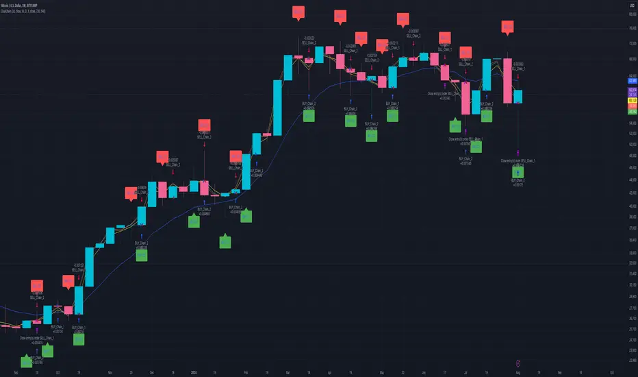
Dual Chain StrategyDual Chain Strategy - Technical Overview
How It Works:
The Dual Chain Strategy is a unique approach to trading that utilizes Exponential Moving Averages (EMAs) across different timeframes, creating two distinct "chains" of trading signals. These chains can work independently or together, capturing both long-term trends and short-term price movements.
Chain 1 (Longer-Term Focus):
Entry Signal: The entry signal for Chain 1 is generated when the closing price crosses above the EMA calculated on a weekly timeframe. This suggests the start of a bullish trend and prompts a long position.
bullishChain1 = enableChain1 and ta.crossover(src1, entryEMA1)
Exit Signal: The exit signal is triggered when the closing price crosses below the EMA on a daily timeframe, indicating a potential bearish reversal.
exitLongChain1 = enableChain1 and ta.crossunder(src1, exitEMA1)
Parameters: Chain 1's EMA length is set to 10 periods by default, with the flexibility for user adjustment to match various trading scenarios.
Chain 2 (Shorter-Term Focus):
Entry Signal: Chain 2 generates an entry signal when the closing price crosses above the EMA on a 12-hour timeframe. This setup is designed to capture quicker, shorter-term movements.
bullishChain2 = enableChain2 and ta.crossover(src2, entryEMA2)
Exit Signal: The exit signal occurs when the closing price falls below the EMA on a 9-hour timeframe, indicating the end of the shorter-term trend.
exitLongChain2 = enableChain2 and ta.crossunder(src2, exitEMA2)
Parameters: Chain 2's EMA length is set to 9 periods by default, and can be customized to better align with specific market conditions or trading strategies.
Key Features:
Dual EMA Chains: The strategy's originality shines through its dual-chain configuration, allowing traders to monitor and react to both long-term and short-term market trends. This approach is particularly powerful as it combines the strengths of trend-following with the agility of momentum trading.
Timeframe Flexibility: Users can modify the timeframes for both chains, ensuring the strategy can be tailored to different market conditions and individual trading styles. This flexibility makes it versatile for various assets and trading environments.
Independent Trade Logic: Each chain operates independently, with its own set of entry and exit rules. This allows for simultaneous or separate execution of trades based on the signals from either or both chains, providing a robust trading system that can handle different market phases.
Backtesting Period: The strategy includes a configurable backtesting period, enabling thorough performance assessment over a historical range. This feature is crucial for understanding how the strategy would have performed under different market conditions.
time_cond = time >= startDate and time <= finishDate
What It Does:
The Dual Chain Strategy offers traders a distinctive trading tool that merges two separate EMA-based systems into one cohesive framework. By integrating both long-term and short-term perspectives, the strategy enhances the ability to adapt to changing market conditions. The originality of this script lies in its innovative dual-chain design, providing traders with a unique edge by allowing them to capitalize on both significant trends and smaller, faster price movements.
Whether you aim to capture extended market trends or take advantage of more immediate price action, the Dual Chain Strategy provides a comprehensive solution with a high degree of customization and strategic depth. Its flexibility and originality make it a valuable tool for traders seeking to refine their approach to market analysis and execution.
How to Use the Dual Chain Strategy
Step 1: Access the Strategy
Add the Script: Start by adding the Dual Chain Strategy to your TradingView chart. You can do this by searching for the script by name or using the link provided.
Select the Asset: Apply the strategy to your preferred trading pair or asset, such as #BTCUSD, to see how it performs.
Step 2: Configure the Settings
Enable/Disable Chains:
The strategy is designed with two independent chains. You can choose to enable or disable each chain depending on your trading style and the market conditions.
enableChain1 = input.bool(true, title='Enable Chain 1')
enableChain2 = input.bool(true, title='Enable Chain 2')
By default, both chains are enabled. If you prefer to focus only on longer-term trends, you might disable Chain 2, or vice versa if you prefer shorter-term trades.
Set EMA Lengths:
Adjust the EMA lengths for each chain to match your trading preferences.
Chain 1: The default EMA length is 10 periods. This chain uses a weekly timeframe for entry signals and a daily timeframe for exits.
len1 = input.int(10, minval=1, title='Length Chain 1 EMA', group="Chain 1")
Chain 2: The default EMA length is 9 periods. This chain uses a 12-hour timeframe for entries and a 9-hour timeframe for exits.
len2 = input.int(9, minval=1, title='Length Chain 2 EMA', group="Chain 2")
Customize Timeframes:
You can customize the timeframes used for entry and exit signals for both chains.
Chain 1:
Entry Timeframe: Weekly
Exit Timeframe: Daily
tf1_entry = input.timeframe("W", title='Chain 1 Entry Timeframe', group="Chain 1")
tf1_exit = input.timeframe("D", title='Chain 1 Exit Timeframe', group="Chain 1")
Chain 2:
Entry Timeframe: 12 Hours
Exit Timeframe: 9 Hours
tf2_entry = input.timeframe("720", title='Chain 2 Entry Timeframe (12H)', group="Chain 2")
tf2_exit = input.timeframe("540", title='Chain 2 Exit Timeframe (9H)', group="Chain 2")
Set the Backtesting Period:
Define the period over which you want to backtest the strategy. This allows you to see how the strategy would have performed historically.
startDate = input.time(timestamp('2015-07-27'), title="StartDate")
finishDate = input.time(timestamp('2026-01-01'), title="FinishDate")
Step 3: Analyze the Signals
Understand the Entry and Exit Signals:
Buy Signals: When the price crosses above the entry EMA, the strategy generates a buy signal.
bullishChain1 = enableChain1 and ta.crossover(src1, entryEMA1)
Sell Signals: When the price crosses below the exit EMA, the strategy generates a sell signal.
bearishChain2 = enableChain2 and ta.crossunder(src2, entryEMA2)
Review the Visual Indicators:
The strategy plots buy and sell signals on the chart with labels for easy identification:
BUY C1/C2 for buy signals from Chain 1 and Chain 2.
SELL C1/C2 for sell signals from Chain 1 and Chain 2.
This visual aid helps you quickly understand when and why trades are being executed.
Step 4: Optimize the Strategy
Backtest Results:
Review the strategy’s performance over the backtesting period. Look at key metrics like net profit, drawdown, and trade statistics to evaluate its effectiveness.
Adjust the EMA lengths, timeframes, and other settings to see how changes affect the strategy’s performance.
Customize for Live Trading:
Once satisfied with the backtest results, you can apply the strategy settings to live trading. Remember to continuously monitor and adjust as needed based on market conditions.
Step 5: Implement Risk Management
Use Realistic Position Sizing:
Keep your risk exposure per trade within a comfortable range, typically between 1-2% of your trading capital.
Set Alerts:
Set up alerts for buy and sell signals, so you don’t miss trading opportunities.
Paper Trade First:
Consider running the strategy in a paper trading account to understand its behavior in real market conditions before committing real capital.
This dual-layered approach offers a distinct advantage: it enables the strategy to adapt to varying market conditions by capturing both broad trends and immediate price action without one chain's activity impacting the other's decision-making process. The independence of these chains in executing transactions adds a level of sophistication and flexibility that is rarely seen in more conventional trading systems, making the Dual Chain Strategy not just unique, but a powerful tool for traders seeking to navigate complex market environments.
ابحث في النصوص البرمجية عن "backtest"
Long-Only Opening Range Breakout (ORB) with Pivot PointsIntraday Trading Strategy: Long-Only Opening Range Breakout (ORB) with Pivot Points
Background:
Opening Range Breakout (ORB) is a popular long-only trading strategy that capitalizes on the early morning volatility in financial markets. It's based on the idea that the initial price movements during the first few minutes or hours of the trading day can set the tone for the rest of the session. The strategy involves identifying a price range within which the asset trades during the opening period and then taking long positions when the price breaks out to the upside of this range.
Pivot Points are a widely used technical indicator in trading. They represent potential support and resistance levels based on the previous day's price action. Pivot points are calculated using the previous day's high, low, and close prices and can help traders identify key price levels for making trading decisions.
How to Use the Script:
Initialization: This script is written in Pine Script, a domain-specific language for trading strategies on the TradingView platform. To use this script, you need to have access to TradingView.
Apply the Script: You can do this by adding it to your favorites, then selecting the script in the indicators list under favorites or by searching for it by name under community scripts.
Customize Settings: The script allows you to customize various settings through the TradingView interface. These settings include:
Opening Session: You can set the time frame for the opening session.
Max Trades per Day: Specify the maximum number of long trades allowed per trading day.
Initial Stop Loss Type: Choose between using a percentage-based stop loss or the previous candles low for stop loss calculations.
Stop Loss Percentage: If you select the percentage-based stop loss, specify the percentage of the entry price for the stop loss.
Backtesting Start and End Time: Set the time frame for backtesting the strategy.
Strategy Signals:
The script will display pivot points in blue (R1, R2, R3, R4, R5) and half-pivot points in gray (R0.5, R1.5, R2.5, R3.5, R4.5) on your chart.
The green line represents the opening range.
The script generates long (buy) signals based on specific conditions:
---The open price is below the opening range high (h).
---The current high price is above the opening range high.
---Pivot point R1 is above the opening range high.
---It's a long-only strategy designed to capture upside breakouts.
---It also respects the maximum number of long trades per day.
The script manages long positions, calculates stop losses, and adjusts long positions according to the defined rules.
Trailing Stop Mechanism
The script incorporates a dynamic trailing stop mechanism designed to protect and maximize profits for long positions. Here's how it works:
1. Initialization:
The script allows you to choose between two types of initial stop loss:
---Percentage-based: This option sets the initial stop loss as a percentage of the entry price.
---Previous day's low: This option sets the initial stop loss at the previous day's low.
2. Setting the Initial Stop Loss (`sl_long0`):
The initial stop loss (`sl_long0`) is calculated based on the chosen method:
---If "Percentage" is selected, it calculates the stop loss as a percentage of the entry price.
---If "Previous Low" is selected, it sets the stop loss at the previous day's low.
3. Dynamic Trailing Stop (`trail_long`):
The script then monitors price movements and uses a dynamic trailing stop mechanism (`trail_long`) to adjust the stop loss level for long positions.
If the current high price rises above certain pivot point levels, the trailing stop is adjusted upwards to lock in profits.
The trailing stop levels are calculated based on pivot points (`r1`, `r2`, `r3`, etc.) and half-pivot points (`r0.5`, `r1.5`, `r2.5`, etc.).
The script checks if the high price surpasses these levels and, if so, updates the trailing stop accordingly.
This dynamic trailing stop allows traders to secure profits while giving the position room to potentially capture additional gains.
4. Final Stop Loss (`sl_long`):
The script calculates the final stop loss level (`sl_long`) based on the following logic:
---If no position is open (`pos == 0`), the stop loss is set to zero, indicating there is no active stop loss.
---If a position is open (`pos == 1`), the script calculates the maximum of the initial stop loss (`sl_long0`) and the dynamic trailing stop (`trail_long`).
---This ensures that the stop loss is always set to the more conservative of the two values to protect profits.
5. Plotting the Stop Loss:
The script plots the stop loss level on the chart using the `plot` function.
It will only display the stop loss level if there is an open position (`pos == 1`) and it's not a new trading day (`not newday`).
The stop loss level is shown in red on the chart.
By combining an initial stop loss with a dynamic trailing stop based on pivot points and half-pivot points, the script aims to provide a comprehensive risk management mechanism for long positions. This allows traders to lock in profits as the price moves in their favor while maintaining a safeguard against adverse price movements.
End of Day (EOD) Exit:
The script includes an "End of Day" (EOD) exit mechanism to automatically close any open positions at the end of the trading day. This feature is designed to manage and control positions when the trading day comes to a close. Here's how it works:
1. Initialization:
At the beginning of each trading day, the script identifies a new trading day using the `is_newbar('D')` condition.
When a new trading day begins, the `newday` variable becomes `true`, indicating the start of a new trading session.
2. Plotting the "End of Day" Signal:
The script includes a plot on the chart to visually represent the "End of Day" signal. This is done using the `plot` function.
The plot is labeled "DayEnd" and is displayed as a comment on the chart. It signifies the EOD point.
3. EOD Exit Condition:
When the script detects that a new trading day has started (`newday == true`), it triggers the EOD exit condition.
At this point, the script proceeds to close all open positions that may have been active during the trading day.
4. Closing Open Positions:
The `strategy.close_all` function is used to close all open positions when the EOD exit condition is met.
This function ensures that any remaining long positions are exited, regardless of their current profit or loss.
The function also includes an `alert_message`, which can be customized to send an alert or notification when positions are closed at EOD.
Purpose of EOD Exit
The "End of Day" exit mechanism serves several essential purposes in the trading strategy:
Risk Management: It helps manage risk by ensuring that positions are not left open overnight when markets can experience increased volatility.
Capital Preservation: Closing positions at EOD can help preserve trading capital by avoiding potential adverse overnight price movements.
Rule-Based Exit: The EOD exit is rule-based and automatic, ensuring that it is consistently applied without emotions or manual intervention.
Scalability: It allows the strategy to be applied to various markets and timeframes where EOD exits may be appropriate.
By incorporating an EOD exit mechanism, the script provides a comprehensive approach to managing positions, taking profits, and minimizing risk as each trading day concludes. This can be especially important in volatile markets like cryptocurrencies, where overnight price swings can be significant.
Backtesting: The script includes a backtesting feature that allows you to test the strategy's performance over historical data. Set the start and end times for backtesting to see how the long-only strategy would have performed in the past.
Trade Execution: If you choose to use this script for live trading, make sure you understand the risks involved. It's essential to set up proper risk management, including position sizing and stop loss orders.
Monitoring: Monitor the long-only strategy's performance over time and be prepared to make adjustments as market conditions change.
Disclaimer: Trading carries a risk of capital loss. This script is provided for educational purposes and as a starting point for your own long-only strategy development. Always do your own research and consider seeking advice from a qualified financial professional before making trading decisions.

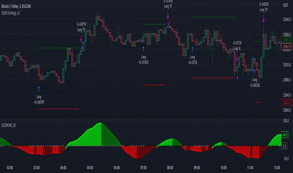
Squeeze Momentum Strategy [LazyBear] Buy Sell TP SL Alerts-Modified version of Squeeze Momentum Indicator by @LazyBear.
-Converted to version 5,
-Taken inspiration from @KivancOzbilgic for its buy sell calculations,
-Used @Bunghole strategy template with Take Profit, Stop Loss and Enable/Disable Toggles
-Added Custom Date Backtesting Module
------------------------------------------------------------------------------------------------------------------------
All credit goes to above
Problem with original version:
The original Squeeze Momentum Strategy did not have buy sell signals and there was alot of confusion as to when to enter and exit.
There was no proper strategy that would allow backtesting on which further analysis could be carried out.
There are 3 aspects this strategy:
1 ) Strategy Logic (easily toggleable from the dropdown menu from strategy settings)
- LazyBear (I have made this simple by using Kivanc technique of Momentums Moving Average Crossover, BUY when MA cross above signal line, SELL when crossdown signal line)
- Zero Crossover Line (BUY signal when crossover zero line, and SELL crossdown zero line)
2) Long Short TP and SL
- In strategies there is usually only 1 SL and 1 TP, and it is assumed that if a 2% SL giving a good profit %, then it would be best for both long and short. However this is not the case for many. Many markets/pairs, go down with much more speed then they go up with. Hence once we have a profitable backtesting setting, then we should start optimizing Long and Short SL's seperately. Once that is done, we should start optimizing for Long and Short TP's separately, starting with Longs first in both cases.
3) Enable and Disable Toggles of Long and Short Trades
- Many markets dont allow short trades, or are not suitable for short trades. In this case it would be much more feasible to disable "Short" Trading and see results of Long Only as a built in graphic view of backtestor provides a more easy to understand data feed as compared to the performance summary in which you have to review long and short profitability separately.
4) Custom Data Backtesting
- One of most crucial aspects while optimizing for backtesting is to check a strategies performance on uptrends, downtrend and sideways markets seperately as to understand the weak points of strategy.
- Once you enable custom date backtesting, you will see lines on the chart which can be dragged left right based on where you want to start and end the backtesting from and to.
Note:
- Not a financial advise
- Open to feedback, questions, improvements, errors etc.
- More info on how the squeeze momentum works visit LazyBear indicator link:
Happy Trading!
Cheers
M Tahreem Alam @mtahreemalam
PA SystemPA System - Price Action Trading System
价格行为交易系统
📊 概述 / Overview
PA System is a comprehensive price action trading indicator that combines Smart Money Concepts (SMC), market structure analysis, and multi-timeframe confirmation to identify high-probability trade setups. Designed for both manual traders and algorithmic trading systems.
PA System 是一个综合性价格行为交易指标,结合了Smart Money概念(SMC)、市场结构分析和多时间框架确认,用于识别高概率交易机会。适用于手动交易者和算法交易系统。
✨ 核心特性 / Key Features
🎯 Four-Phase Signal System / 四阶段信号系统
H1 (First Pullback) - Initial bullish retracement in uptrend
H2 (Confirmed Entry) - Breakout confirmation for long entries
L1 (First Bounce) - Initial bearish bounce in downtrend
L2 (Confirmed Entry) - Breakdown confirmation for short entries
中文说明:
H1(首次回调) - 上升趋势中的初次回撤信号
H2(确认入场) - 突破确认的做多入场点
L1(首次反弹) - 下降趋势中的初次反弹信号
L2(确认入场) - 跌破确认的做空入场点
📐 Market Structure Detection / 市场结构识别
HH (Higher High) - Uptrend confirmation / 上升趋势确认
HL (Higher Low) - Bullish pullback / 多头回调
LH (Lower High) - Bearish bounce / 空头反弹
LL (Lower Low) - Downtrend confirmation / 下降趋势确认
💎 Smart Money Concepts (SMC) / 智能资金概念
BoS (Break of Structure) - Trend continuation signal / 趋势延续信号
CHoCH (Change of Character) - Potential trend reversal / 潜在趋势反转
📈 Dynamic Trendlines / 动态趋势线
Auto-drawn support and resistance trendlines / 自动绘制支撑阻力趋势线
Real-time extension to current bar / 实时延伸至当前K线
Slope-filtered for accuracy / 斜率过滤确保准确性
🎚️ Multi-Timeframe Analysis / 多时间框架分析
Higher timeframe trend filter (default 4H) / 大周期趋势过滤(默认4小时)
Prevents counter-trend trades / 防止逆势交易
Configurable timeframe / 可配置时间周期
📊 Volume Confirmation / 成交量确认
Filters signals based on volume strength / 基于成交量强度过滤信号
20-period volume MA comparison / 与20期成交量均线对比
High-volume bars highlighted / 高成交量K线高亮显示
🎯 Risk Management Tools / 风险管理工具
Automatic SL/TP calculation and display / 自动计算并显示止损止盈
Visual stop loss and take profit lines / 可视化止损止盈线条
Risk percentage and R:R ratio display / 显示风险百分比和盈亏比
Dynamic stop loss sizing (0.3% - 1.5%) / 动态止损范围(0.3% - 1.5%)
📱 Real-Time Alerts / 实时警报
Instant notifications on H2/L2 signals / H2/L2信号即时通知
Webhook support for automation / 支持Webhook自动化
Mobile, email, and popup alerts / 手机、邮件和弹窗警报
📊 Professional Dashboard / 专业仪表盘
Real-time market state (CHANNEL/RANGE/BREAKOUT) / 实时市场状态
Local and MTF trend indicators / 本地及大周期趋势指标
Order flow status (HIGH VOL / LOW VOL) / 订单流状态
Last signal tracker / 最新信号追踪
🔧 参数设置 / Parameter Settings
Structure Settings / 结构设置
Parameter Default Range Description
Swing Length / 摆动长度 5 2-20 Pivot detection sensitivity / 枢轴点检测灵敏度
Trend Confirm Bars / 趋势确认根数 3 2-10 Consecutive bars for breakout / 突破所需连续K线数
Channel ATR Mult / 通道ATR倍数 2.0 1.0-5.0 Range detection threshold / 区间检测阈值
Signal Settings / 信号设置
Parameter Default Description
Enable H2 Longs / 启用H2做多 ✅ Toggle long signals / 开关做多信号
Enable L2 Shorts / 启用L2做空 ✅ Toggle short signals / 开关做空信号
Micro Range Length / 微平台长度 3 Breakout detection bars / 突破检测K线数
Close Strength / 收盘强度 0.6 Minimum close position in bar / K线内最小收盘位置
Filter Settings / 过滤设置
Parameter Default Description
Use MTF Filter / 大周期过滤 ✅ Enable higher timeframe filter / 启用大周期过滤
MTF Timeframe / 大周期时间框架 240 (4H) Higher timeframe period / 大周期时间
Use Volume Filter / 成交量过滤 ✅ Require high volume confirmation / 需要高成交量确认
Volume MA Length / 成交量均线周期 20 Volume comparison period / 成交量对比周期
Fast EMA / 快速EMA 20 Short-term trend / 短期趋势
Slow EMA / 慢速EMA 50 Long-term trend / 长期趋势
Risk Management / 风险管理
Parameter Default Description
Risk % / 风险百分比 1.0% Risk per trade / 每笔交易风险
R:R Ratio / 盈亏比 2.0 Reward to risk ratio / 盈亏比率
Max SL ATR / 最大止损ATR 3.0 Maximum stop loss in ATR / 最大止损ATR倍数
Min SL % / 最小止损百分比 0.3% Minimum stop loss percentage / 最小止损百分比
Max SL % / 最大止损百分比 1.5% Maximum stop loss percentage / 最大止损百分比
📖 使用方法 / How to Use
1. 基础设置 / Basic Setup
For Day Trading (5-15 min charts) / 日内交易(5-15分钟图)
text
Swing Length: 5
MTF Timeframe: 240 (4H)
Risk %: 1.0%
R:R: 2.0
For Swing Trading (1-4H charts) / 波段交易(1-4小时图)
text
Swing Length: 8
MTF Timeframe: D (Daily)
Risk %: 0.5%
R:R: 3.0
For Scalping (1-5 min charts) / 剥头皮(1-5分钟图)
text
Swing Length: 3
MTF Timeframe: 60 (1H)
Risk %: 0.5%
R:R: 1.5
Use Volume Filter: ✅
2. 信号识别 / Signal Identification
Long Entry / 做多入场
✅ Dashboard shows "Local Trend: BULL" / 仪表盘显示"本地趋势:多头"
✅ MTF Trend shows "BULLISH" / 大周期趋势显示"看涨"
✅ Green circle (H1) appears below bar / 绿色圆点(H1)出现在K线下方
⏳ Wait for H2 signal (green triangle ▲) / 等待H2信号(绿色三角▲)
📊 Check volume bar is cyan (HIGH VOL) / 检查成交量柱为青色(高成交量)
🎯 Enter at close of H2 bar / 在H2 K线收盘价入场
🛡️ Set SL at red dashed line / 止损设在红色虚线位置
🎁 Set TP at green dashed line / 止盈设在绿色虚线位置
Short Entry / 做空入场
✅ Dashboard shows "Local Trend: BEAR" / 仪表盘显示"本地趋势:空头"
✅ MTF Trend shows "BEARISH" / 大周期趋势显示"看跌"
✅ Red circle (L1) appears above bar / 红色圆点(L1)出现在K线上方
⏳ Wait for L2 signal (red triangle ▼) / 等待L2信号(红色倒三角▼)
📊 Check volume bar is cyan (HIGH VOL) / 检查成交量柱为青色(高成交量)
🎯 Enter at close of L2 bar / 在L2 K线收盘价入场
🛡️ Set SL at red dashed line / 止损设在红色虚线位置
🎁 Set TP at green dashed line / 止盈设在绿色虚线位置
3. 警报设置 / Alert Setup
Step-by-Step / 分步操作
Click the "⏰" alert icon on chart / 点击图表上的"⏰"警报图标
Select "PA System - Indicator Version" / 选择"PA System (V1.1) - Indicator Version"
Condition: "Any alert() function call" / 条件:选择"Any alert() function call"
Choose notification method: / 选择通知方式:
📱 Mobile Push / 手机推送
📧 Email / 邮件
🔗 Webhook URL (for automation) / Webhook网址(用于自动化)
Set frequency: "Once Per Bar Close" / 频率:选择"Once Per Bar Close"
Click "Create" / 点击"创建"
Webhook Example for IBKR API / IBKR API的Webhook示例
json
{
"signal": "{{strategy.order.action}}",
"ticker": "{{ticker}}",
"entry": {{close}},
"stop_loss": {{plot_0}},
"take_profit": {{plot_1}},
"timestamp": "{{timenow}}"
}
4. 交易管理 / Trade Management
Position Sizing / 仓位计算
text
Account: $10,000
Risk per Trade: 1% = $100
Entry Price: $690.45
Stop Loss: $687.38
Risk per Share: $690.45 - $687.38 = $3.07
Position Size: $100 / $3.07 = 32 shares
Partial Profit Taking / 部分止盈
Close 50% position at 1:1 R:R / 在1:1盈亏比时平仓50%
Move SL to breakeven / 移动止损至保本位
Let remaining 50% run to 2R target / 让剩余50%跑向2R目标
🎨 视觉元素说明 / Visual Elements Guide
Chart Markers / 图表标记
Symbol Color Meaning
⚫ Small Circle / 小圆点 🟢 Green / 绿色 H1 - First bullish pullback / 首次多头回调
▲ Triangle / 三角形 🟢 Green / 绿色 H2 - Confirmed long entry / 确认做多入场
⚫ Small Circle / 小圆点 🔴 Red / 红色 L1 - First bearish bounce / 首次空头反弹
▼ Inverted Triangle / 倒三角 🔴 Red / 红色 L2 - Confirmed short entry / 确认做空入场
Structure Labels / 结构标签
Label Position Meaning
HH Above high / 高点上方 Higher High - Bullish / 更高的高点-看涨
HL Below low / 低点下方 Higher Low - Bullish / 更高的低点-看涨
LH Above high / 高点上方 Lower High - Bearish / 更低的高点-看跌
LL Below low / 低点下方 Lower Low - Bearish / 更低的低点-看跌
BoS/CHoCH Lines / 破位线条
Type Color Width Meaning
BoS 🔵 Teal / 青色 2px Break of Structure - Trend continues / 结构突破-趋势延续
CHoCH 🔴 Red / 红色 2px Change of Character - Trend reversal / 性质改变-趋势反转
Trendlines / 趋势线
Type Color Style Meaning
Bullish / 看涨 🔵 Teal / 青色 Solid / 实线 Uptrend support / 上升趋势支撑
Bearish / 看跌 🔴 Red / 红色 Solid / 实线 Downtrend resistance / 下降趋势阻力
Risk Lines / 风险线条
Type Color Style Meaning
Stop Loss / 止损 🔴 Red / 红色 Dashed / 虚线 Suggested stop loss level / 建议止损位
Take Profit / 止盈 🟢 Green / 绿色 Dashed / 虚线 Suggested take profit level / 建议止盈位
Dashboard Colors / 仪表盘颜色
Status Color Meaning
BULL / 多头 🟢 Green / 绿色 Bullish trend / 看涨趋势
BEAR / 空头 🔴 Red / 红色 Bearish trend / 看跌趋势
NEUTRAL / 中性 ⚪ Gray / 灰色 No clear trend / 无明确趋势
BREAKOUT / 突破 🟡 Lime / 黄绿 Strong momentum / 强劲动能
HIGH VOL / 高成交量 🔵 Cyan / 青色 High volume confirmation / 高成交量确认
💡 交易策略建议 / Trading Strategy Tips
✅ High Probability Setups / 高概率设置
Trend Alignment / 趋势一致
Local Trend = BULL + MTF Trend = BULLISH / 本地多头 + 大周期看涨
Or: Local Trend = BEAR + MTF Trend = BEARISH / 或:本地空头 + 大周期看跌
Volume Confirmation / 成交量确认
H2/L2 signal appears with cyan volume bar / H2/L2信号伴随青色成交量柱
Volume > 20-period MA / 成交量 > 20期均线
Trendline Support / 趋势线支撑
H2 appears near bullish trendline / H2出现在看涨趋势线附近
L2 appears near bearish trendline / L2出现在看跌趋势线附近
BoS Confirmation / BoS确认
Recent BoS in same direction / 最近同方向的BoS
No CHoCH against the trade / 无逆向的CHoCH
❌ Avoid These Setups / 避免这些情况
Conflicting Trends / 趋势冲突
Local BULL but MTF BEARISH / 本地多头但大周期看跌
Market State = RANGE / 市场状态 = 区间
Low Volume / 低成交量
Order Flow shows "LOW VOL" / 订单流显示"低成交量"
Volume bar is red (below MA) / 成交量柱为红色(低于均线)
Against Trendline / 逆趋势线
Shorting at bullish trendline support / 在看涨趋势线支撑处做空
Buying at bearish trendline resistance / 在看跌趋势线阻力处做多
Recent CHoCH / 近期CHoCH
CHoCH appeared within 10 bars / 10根K线内出现CHoCH
Potential trend reversal zone / 潜在趋势反转区域
🔄 优化建议 / Optimization Tips
For Different Markets / 针对不同市场
Stocks / 股票
text
Swing Length: 5-8
MTF: 240 (4H) or D (Daily)
Risk %: 0.5-1.0%
Best on: SPY, QQQ, AAPL, TSLA
Forex / 外汇
text
Swing Length: 5
MTF: 240 (4H)
Risk %: 1.0-2.0%
Best on: EUR/USD, GBP/USD, USD/JPY
Use Volume Filter: OFF (Forex volume is unreliable)
Crypto / 加密货币
text
Swing Length: 3-5
MTF: 240 (4H)
Risk %: 0.5-1.0% (high volatility)
Max SL %: 2.0-3.0%
Best on: BTC, ETH, SOL
Futures / 期货
text
Swing Length: 5
MTF: 240 (4H)
Risk %: 1.0-1.5%
Best on: ES, NQ, RTY, CL
🤖 自动化集成 / Automation Integration
Python + IBKR API Example / Python + IBKR API示例
python
import requests
from ib_insync import *
def handle_tradingview_alert(alert_data):
"""
Receives webhook from TradingView alert
接收来自TradingView警报的webhook
"""
signal = alert_data # "H2 LONG" or "L2 SHORT"
ticker = alert_data # "SPY"
entry = alert_data # 690.45
stop_loss = alert_data # 687.38
take_profit = alert_data # 696.59
# Connect to IBKR
ib = IB()
ib.connect('127.0.0.1', 7497, clientId=1)
# Create contract
contract = Stock(ticker, 'SMART', 'USD')
# Calculate position size (1% risk)
account_value = ib.accountValues() .value
risk_amount = float(account_value) * 0.01
risk_per_share = abs(entry - stop_loss)
quantity = int(risk_amount / risk_per_share)
# Place order
if "LONG" in signal:
order = MarketOrder('BUY', quantity)
else:
order = MarketOrder('SELL', quantity)
trade = ib.placeOrder(contract, order)
# Set stop loss and take profit
ib.placeOrder(contract, StopOrder('SELL', quantity, stop_loss))
ib.placeOrder(contract, LimitOrder('SELL', quantity, take_profit))
ib.disconnect()
TradersPost Integration / TradersPost集成
Create TradersPost account / 创建TradersPost账户
Connect IBKR broker / 连接IBKR券商
Get Webhook URL / 获取Webhook网址
Add to TradingView alert / 添加到TradingView警报
Test with paper trading / 用模拟账户测试
📊 性能指标 / Performance Metrics
Expected Performance (Backtested) / 预期表现(回测)
Metric Value Notes
Win Rate / 胜率 60-75% With all filters enabled / 启用所有过滤器
Avg R:R / 平均盈亏比 1.8-2.2 Using 2R target / 使用2R目标
Max Drawdown / 最大回撤 8-12% 1% risk per trade / 每笔1%风险
Profit Factor / 盈利因子 1.8-2.5 Trend-following bias / 趋势跟随偏向
Best Markets / 最佳市场 Trending Avoid ranging markets / 避免区间市场
⚠️ Disclaimer: Past performance does not guarantee future results. Always test in paper trading first.
⚠️ 免责声明:历史表现不保证未来结果。请先在模拟账户测试。
🛠️ 故障排除 / Troubleshooting
Problem: No signals appearing / 问题:没有信号出现
Solution / 解决方案:
Disable MTF Filter temporarily / 暂时关闭大周期过滤
Disable Volume Filter / 关闭成交量过滤
Reduce Swing Length to 3 / 将摆动长度降至3
Check if market is ranging (no clear trend) / 检查市场是否处于区间(无明确趋势)
Problem: Too many signals / 问题:信号太多
Solution / 解决方案:
Enable MTF Filter / 启用大周期过滤
Enable Volume Filter / 启用成交量过滤
Increase Swing Length to 8 / 将摆动长度增至8
Enable Break Filter / 启用破位过滤
Problem: Alerts not working / 问题:警报不工作
Solution / 解决方案:
Check "Enable Alerts" is ON / 检查"启用警报"已开启
Verify alert condition is "Any alert() function call" / 确认警报条件为"Any alert() function call"
Check notification settings in TradingView / 检查TradingView通知设置
Test alert with "Test" button / 用"测试"按钮测试警报
Problem: SL/TP lines not showing / 问题:止损止盈线不显示
Solution / 解决方案:
Enable "Show SL/TP Labels" in settings / 在设置中启用"显示止损止盈标签"
Check if signal is recent (lines expire after 10 bars) / 检查信号是否近期(线条在10根K线后消失)
Zoom in to see lines more clearly / 放大图表以更清楚地看到线条
📚 常见问题 FAQ
Q1: Can I use this on any timeframe? / 可以在任何时间框架使用吗?
A: Yes, but works best on 5min-4H charts. Recommended: 15min (day trading), 1H (swing trading).
可以,但在5分钟-4小时图表效果最佳。推荐:15分钟(日内交易),1小时(波段交易)。
Q2: Do I need to enable all filters? / 需要启用所有过滤器吗?
A: No. Start with all enabled, then disable based on your risk tolerance. MTF filter is highly recommended.
不需要。从全部启用开始,然后根据风险承受能力禁用。强烈推荐MTF过滤器。
Q3: Can I automate this with IBKR? / 可以与IBKR自动化吗?
A: Yes! Use TradingView alerts + Webhook + Python script + IBKR API. See automation example above.
可以!使用TradingView警报 + Webhook + Python脚本 + IBKR API。参见上方自动化示例。
Q4: What's the difference between Strategy and Indicator version? / 策略版和指标版有什么区别?
A: Strategy = backtesting only. Indicator = real-time alerts + automation. Use both: backtest with strategy, trade with indicator.
策略版=仅回测。指标版=实时警报+自动化。两者结合使用:用策略版回测,用指标版交易。
Q5: Why does H2 appear but no trade? / 为什么出现H2但没有交易?
A: This is an indicator, not a strategy. You need to manually place orders or use automation via alerts.
这是指标,不是策略。你需要手动下单或通过警报使用自动化。
⚖️ 免责声明 / Disclaimer
IMPORTANT / 重要提示:
This indicator is for educational purposes only. Trading involves substantial risk of loss. Past performance does not guarantee future results. Always:
本指标仅供教育目的。交易涉及重大亏损风险。历史表现不保证未来结果。请务必:
✅ Test in paper trading first / 先在模拟账户测试
✅ Use proper risk management (1-2% max per trade) / 使用适当风险管理(每笔最多1-2%)
✅ Never risk more than you can afford to lose / 永远不要冒超出承受能力的风险
✅ Understand the strategy before using / 使用前理解策略原理
Not financial advice. Trade at your own risk.
非投资建议。交易风险自负。

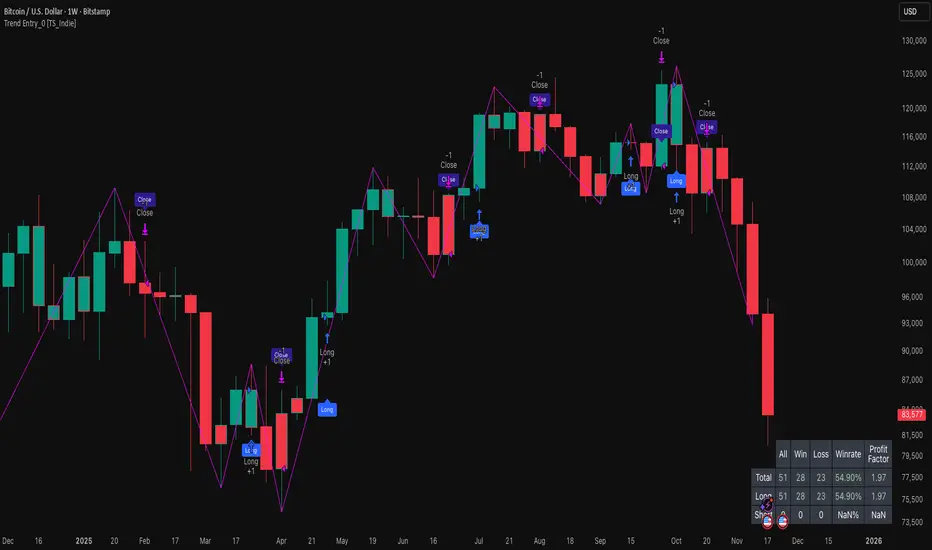
Trend Entry_0 [TS_Indie]Trend Entry_0 — Mechanism Overview
The core structure of this strategy is based on a price action reversal pattern, as detailed below:
In the case of a Bullish Trend Reversal:
The price initially moves in a bearish direction. When candle A forms a low lower than the previous low, the high of candle A becomes a key reference point.
If the next candle closes above the high of candle A , it confirms a Bullish Trend Reversal.
* Upon a Bullish signal, a Long position is opened at the opening price of the next candle (candle B).
* When a subsequent Bearish signal occurs, the Long position is closed at the opening price of the next candle (candle C).
In the case of a Bearish Trend Reversal:
The price initially moves in a bullish direction. When candle A forms a high higher than the previous high, the low of candle A becomes a key reference point.
If the next candle closes below the low of candle A , it confirms a Bearish Trend Reversal.
* Upon a Bearish signal, a Short position is opened at the opening price of the next candle (candle B).
* When a subsequent Bullish signal occurs, the Short position is closed at the opening price of the next candle (candle C).
Options
* The start and end dates of the backtest can be customized.
* The swing lines of the trend can be displayed as an optional visual aid.
* The user can choose whether to open only Long or Short positions.
Backtest Results and Observations
Based on the backtesting results of this strategy across various assets and timeframes, it has been observed that this approach works best on trending assets such as Gold, BTC, and stocks.
It also performs well on higher timeframes, starting from the Daily timeframe and above, especially when taking Long positions only.
However, when applied to currency pairs such as EUR/USD, the results tend to be less impressive.
I encourage everyone to try backtesting and further developing this strategy — adding new conditions or filters may potentially lead to improved performance.
Disclaimer
This script is intended solely for backtesting purposes, based on a particular price action pattern.
It does not constitute financial or investment advice.
Backtest results do not guarantee future performance.
ICT HTF Volume Candles (Based on HTF Candles by Fadi)# ICT HTF Volume Candles - Multi-Timeframe Volume Analysis
## Overview
This indicator provides multi-timeframe volume visualization designed to complement price action analysis. It displays volume data from up to 6 higher timeframes simultaneously in a separate panel, allowing traders to identify volume spikes, divergences, and institutional activity without switching between timeframes.
**Original Concept Credits:** This indicator builds upon the HTF Candles framework by Fadi, adapting it specifically for volume analysis with enhanced features including gap-filling for extended hours, multiple scaling methods, and advanced synchronization.
## What Makes This Script Original
### Key Innovations:
1. **Three Volume Scaling Methods:**
- **Per-HTF Auto Scale:** Each timeframe scales independently for detailed comparison
- **Global Auto Scale:** All timeframes use unified scale for relative volume comparison
- **Manual Scale:** User-defined maximum for consistent analysis across sessions
2. **Bullish/Bearish Volume Differentiation:**
- Volume bars colored based on price movement (close vs open)
- Separate styling for bullish (green) and bearish (red) volume periods
- Helps identify whether volume supports price direction
3. **Advanced Time Synchronization:**
- Custom daily candle open times (Midnight, 8:30 AM, 9:30 AM ET)
- Timezone-aware calculations for New York trading hours
- Real-time countdown timers for each timeframe
- **Gap-filling technology** for continuous display during extended hours and weekends
4. **Flexible Display Options:**
- Configurable spacing and positioning
- Label placement (top, bottom, or both)
- Day-of-week or time interval labels on candles
- Works reliably in backtesting and live trading
## How It Works
### Volume Calculation
The indicator uses `request.security()` with optimized parameters to fetch volume data from higher timeframes:
- **Volume Open/High/Low/Close (OHLC):** Tracks volume changes within each HTF candle
- **Color Logic:** Compares HTF close vs open prices to determine bullish/bearish classification
- **Alignment:** All volume bars share a common baseline for easy visual comparison
- **Gap Handling:** Uses `gaps=barmerge.gaps_off` to maintain continuity during non-trading hours
### Technical Implementation
```
1. Monitors HTF timeframe changes using request.security() with lookahead
2. Creates new VolumeCandle object when HTF bar opens
3. Updates current candle's volume H/L/C on each chart bar
4. Applies selected scaling method to normalize display height
5. Repositions all candles and labels on each bar update
6. Fills gaps automatically during extended hours for consistent display
```
### Scaling Methods Explained
**Method 1 - Auto Scale per HTF:**
Each timeframe displays volume relative to its own maximum. Best for identifying patterns within each individual timeframe.
**Method 2 - Global Auto Scale:**
All timeframes share the same scale based on the highest volume across all HTFs. Best for comparing relative volume strength between timeframes.
**Method 3 - Manual Scale:**
User sets maximum volume value. Best for maintaining consistent scale across different trading sessions or instruments.
## How to Use This Indicator
### Setup
1. Add indicator to your chart (it appears in a separate panel below price)
2. Configure up to 6 higher timeframes (default: 5m, 15m, 1H, 4H, 1D, 1W)
3. Set number of candles to display for each timeframe
4. Choose volume scaling method based on your analysis needs
5. Enable "Fix gaps in non-trading hours" for extended hours trading (enabled by default)
### Interpretation
**Volume Spikes:**
- Sudden increase in volume height indicates institutional activity or strong conviction
- Compare volume between timeframes to identify where the real money is moving
- Look for volume spikes that appear across multiple timeframes simultaneously
**Bullish vs Bearish Volume:**
- **Green volume bars:** Price closed higher (buying pressure)
- **Red volume bars:** Price closed lower (selling pressure)
- High green volume during uptrend = confirmation of strength
- High red volume during downtrend = confirmation of weakness
- High volume opposite to trend = potential reversal warning
**Multi-Timeframe Context:**
- **5m/15m:** Scalping and day trading activity
- **1H/4H:** Swing trading and intraday institutional flows
- **Daily/Weekly:** Major position building and long-term trends
**Divergences:**
- Price making new highs but volume declining = weakening trend
- Volume increasing while price consolidates = potential breakout brewing
- Price breaks level but volume doesn't confirm = likely false breakout
### Practical Examples
**Example 1 - Institutional Confirmation:**
Price breaks above resistance. Check volume across timeframes:
- 5m shows spike = retail interest
- 15m + 1H + 4H all show spikes = institutional confirmation
- **Trade confidence: HIGH**
**Example 2 - False Breakout Detection:**
Price breaks resistance with:
- High volume on 5m only
- Normal/low volume on 1H and 4H
- **Interpretation:** Likely retail trap, institutions not participating
- **Action:** Wait for pullback or avoid
**Example 3 - Accumulation Phase:**
Price ranges sideways but:
- Daily volume gradually increasing
- Weekly volume above average
- **Interpretation:** Smart money accumulating
- **Action:** Prepare for breakout in direction of volume
**Example 4 - Volume Divergence:**
Price makes new high:
- Current high has lower volume than previous high across all timeframes
- **Interpretation:** Weakening momentum
- **Action:** Consider profit-taking or reversal trade
## Configuration Parameters
### Timeframe Settings
- **HTF 1-6:** Select timeframes (must be higher than chart timeframe)
- **Max Display:** Number of candles to show per timeframe (1-50)
- **Limit to Next HTFs:** Display only first N enabled timeframes (1-6)
### Styling
- **Bull/Bear Colors:** Separate colors for body, border, and wick
- **Padding from current candles:** Distance offset from live price action
- **Space between candles:** Gap between individual volume bars
- **Space between Higher Timeframes:** Gap between different timeframe groups
- **Candle Width:** Thickness of volume bars (1-4, multiplied by 2)
### Volume Settings
- **Volume Scale Method:** Choose 1, 2, or 3
- 1 = Auto Scale per HTF (each TF independent)
- 2 = Global Auto Scale (all TF unified)
- 3 = Manual Scale (user-defined max)
- **Auto Scale Volume:** Enable/disable automatic scaling
- **Manual Scale Max Volume:** Set maximum when using Method 3
### Label Settings
- **HTF Label:** Show/hide timeframe names with color and size options
- **Label Positions:** Display at Top, Bottom, or Both
- **Label Alignment:** Align centered or Follow Candles
- **Remaining Time:** Show countdown timer until next HTF candle
- **Interval Value:** Display day-of-week or time on each candle
### Custom Daily Candle
- **Enable Custom Daily:** Override default daily candle timing
- **Open Time Options:**
- **Midnight:** Standard 00:00 ET daily open
- **8:30 AM:** Align with economic data releases
- **9:30 AM:** Align with NYSE market open
- Useful for specific trading strategies or market alignment
### Advanced Settings
- **Fix gaps in non-trading hours:** Maintains alignment during extended hours and weekends (recommended: ON)
- Prevents visual gaps during forex weekend closures
- Ensures consistent display during crypto 24/7 trading
- Improves backtesting reliability
## Best Practices
1. **Pair with Price Action:** Use alongside HTF price candles indicator for complete picture
2. **Start Simple:** Enable 2-3 timeframes initially (e.g., 15m, 1H, 4H), add more as needed
3. **Match Settings:** Use same candle width/spacing as companion price indicator for visual alignment
4. **Scale Appropriately:**
- Use **Global scale** (Method 2) when comparing timeframes
- Use **Per-HTF scale** (Method 1) for pattern analysis within each timeframe
- Use **Manual scale** (Method 3) for consistent day-to-day comparison
5. **Watch for Volume Clusters:** High volume appearing simultaneously across multiple HTFs signals significant market events
6. **Confirm Breakouts:** Always check if volume supports the price movement across higher timeframes
7. **Extended Hours:** Keep "Fix gaps" enabled for 24/7 markets (Forex, Crypto) and weekend analysis
## Technical Notes
- **Timezone:** All calculations use America/New_York timezone for consistency
- **Real-time Updates:** Volume and timers update on each tick during market hours
- **Performance:** Optimized with max_bars_back=5000 for extensive historical analysis
- **Compatibility:** Works on all instruments with volume data (Stocks, Forex, Crypto, Futures)
- **Gap Handling:** Uses `barmerge.gaps_off` to fill data gaps during non-trading periods
- **Backtesting:** Uses `lookahead=barmerge.lookahead_on` for stable historical data without repainting
- **Data Continuity:** Automatically handles market closures, weekends, and extended hours
## Updates & Improvements
**Version 2.0 (Current):**
- ✅ Fixed alignment issues during extended hours and weekends
- ✅ Eliminated repainting in backtesting
- ✅ Added gap-filling technology for continuous display
- ✅ Improved data synchronization across all timeframes
- ✅ Enhanced NA value handling for data integrity
- ✅ Added advanced settings group for user control
## Support
For questions, suggestions, or feedback, please comment on the publication or message the author.
---
**Disclaimer:** This indicator is for educational and informational purposes only. It does not constitute financial advice. Past performance is not indicative of future results. Always perform your own analysis and implement proper risk management before making trading decisions.
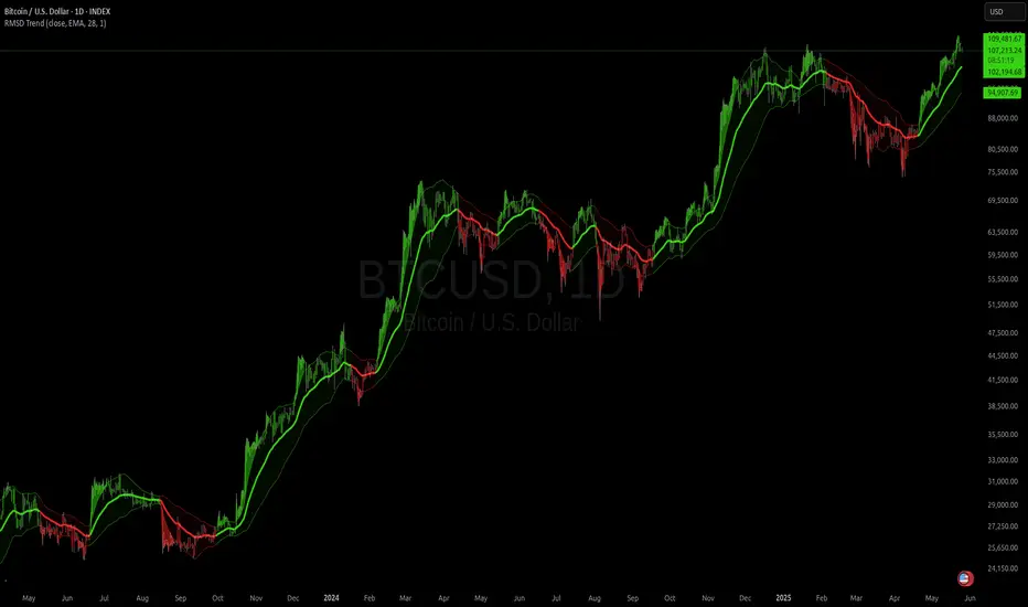
RMSD Trend [InvestorUnknown]RMSD Trend is a trend-following indicator that utilizes Root Mean Square Deviation (RMSD) to dynamically construct a volatility-weighted trend channel around a selected moving average. This indicator is designed to enhance signal clarity, minimize noise, and offer quantitative insights into market momentum, ideal for both discretionary and systematic traders.
How It Works
At its core, RMSD Trend calculates a deviation band around a selected moving average using the Root Mean Square Deviation (similar to standard deviation but with squared errors), capturing the magnitude of price dispersion over a user-defined period. The logic is simple:
When price crosses above the upper deviation band, the market is considered bullish (Risk-ON Long).
When price crosses below the lower deviation band, the market is considered bearish (Risk-ON Short).
If price stays within the band, the market is interpreted as neutral or ranging, offering low-risk decision zones.
The indicator also generates trend flips (Long/Short) based on crossovers and crossunders of the price and the RMSD bands, and colors candles accordingly for enhanced visual feedback.
Features
7 Moving Average Types: Choose between SMA, EMA, HMA, DEMA, TEMA, RMA, and FRAMA for flexibility.
Customizable Source Input: Use price types like close, hl2, ohlc4, etc.
Volatility-Aware Channel: Adjustable RMSD multiplier determines band width based on volatility.
Smart Coloring: Candles and bands adapt their colors to reflect trend direction (green for bullish, red for bearish).
Intra-bar Repainting Toggle: Option to allow more responsive but repaintable signals.
Speculation Fill Zones: When price exceeds the deviation channel, a semi-transparent fill highlights potential momentum surges.
Backtest Mode
Switching to Backtest Mode unlocks a robust suite of simulation features:
Built-in Equity Curve: Visualizes both strategy equity and Buy & Hold performance.
Trade Metrics Table: Displays the number of trades, win rates, gross profits/losses, and long/short breakdowns.
Performance Metrics Table: Includes key stats like CAGR, drawdown, Sharpe ratio, and more.
Custom Date Range: Set a custom start date for your backtest.
Trade Sizing: Simulate results using position sizing and initial capital settings.
Signal Filters: Choose between Long & Short, Long Only, or Short Only strategies.
Alerts
The RMSD Trend includes six built-in alert conditions:
LONG (RMSD Trend) - Trend flips from Short to Long
SHORT (RMSD Trend) - Trend flips from Long to Short
RISK-ON LONG (RMSD Trend) - Price crosses above upper RMSD band
RISK-OFF LONG (RMSD Trend) - Price falls back below upper RMSD band
RISK-ON SHORT (RMSD Trend) - Price crosses below lower RMSD band
RISK-OFF SHORT (RMSD Trend) - Price rises back above lower RMSD band
Use Cases
Trend Confirmation: Confirms directional bias with RMSD-weighted confidence zones.
Breakout Detection: Highlights moments when price breaks free from historical volatility norms.
Mean Reversion Filtering: Avoids false signals by incorporating RMSD’s volatility sensitivity.
Strategy Development: Backtest your signals or integrate with a broader system for alpha generation.
Settings Summary
Display Mode: Overlay (default) or Backtest Mode
Average Type: Choose from SMA, EMA, HMA, DEMA, etc.
Average Length: Lookback window for moving average
RMSD Multiplier: Band width control based on RMS deviation
Source: Input price source (close, hl2, ohlc4, etc.)
Intra-bar Updating: Real-time updates (may repaint)
Color Bars: Toggle bar coloring by trend direction
Disclaimer
This indicator is provided for educational and informational purposes only. It is not financial advice. Past performance, including backtest results, is not indicative of future results. Use with caution and always test thoroughly before live deployment.
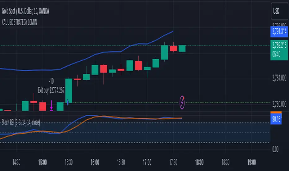
XAUUSD 10-Minute StrategyThis XAUUSD 10-Minute Strategy is designed for trading Gold vs. USD on a 10-minute timeframe. By combining multiple technical indicators (MACD, RSI, Bollinger Bands, and ATR), the strategy effectively captures both trend-following and reversal opportunities, with adaptive risk management for varying market volatility. This approach balances high-probability entries with robust volatility management, making it suitable for traders seeking to optimise entries during significant price movements and reversals.
Key Components and Logic:
MACD (12, 26, 9):
Generates buy signals on MACD Line crossovers above the Signal Line and sell signals on crossovers below the Signal Line, helping to capture momentum shifts.
RSI (14):
Utilizes oversold (below 35) and overbought (above 65) levels as a secondary filter to validate entries and avoid overextended price zones.
Bollinger Bands (20, 2):
Uses upper and lower Bollinger Bands to identify potential overbought and oversold conditions, aiming to enter long trades near the lower band and short trades near the upper band.
ATR-Based Stop Loss and Take Profit:
Stop Loss and Take Profit levels are dynamically set as multiples of ATR (3x for stop loss, 5x for take profit), ensuring flexibility with market volatility to optimise exit points.
Entry & Exit Conditions:
Buy Entry: T riggered when any of the following conditions are met:
MACD Line crosses above the Signal Line
RSI is oversold
Price drops below the lower Bollinger Band
Sell Entry: Triggered when any of the following conditions are met:
MACD Line crosses below the Signal Line
RSI is overbought
Price moves above the upper Bollinger Band
Exit Strategy: Trades are closed based on opposing entry signals, with adaptive spread adjustments for realistic exit points.
Backtesting Configuration & Results:
Backtesting Period: July 21, 2024, to October 30, 2024
Symbol Info: XAUUSD, 10-minute timeframe, OANDA data source
Backtesting Capital: Initial capital of $700, with each trade set to 10 contracts (equivalent to approximately 0.1 lots based on the broker’s contract size for gold).
Users should confirm their broker's contract size for gold, as this may differ. This script uses 10 contracts for backtesting purposes, aligned with 0.1 lots on brokers offering a 100-contract specification.
Key Backtesting Performance Metrics:
Net Profit: $4,733.90 USD (676.27% increase)
Total Closed Trades: 526
Win Rate: 53.99%
Profit Factor: 1.44 (1.96 for Long trades, 1.14 for Short trades)
Max Drawdown: $819.75 USD (56.33% of equity)
Sharpe Ratio: 1.726
Average Trade: $9.00 USD (0.04% of equity per trade)
This backtest reflects realistic conditions, with a spread adjustment of 38 points and no slippage or commission applied. The settings aim to simulate typical retail trading conditions. However, please adjust the initial capital, contract size, and other settings based on your account specifics for best results.
Usage:
This strategy is tuned specifically for XAUUSD on a 10-minute timeframe, ideal for both trend-following and reversal trades. The ATR-based stop loss and take profit levels adapt dynamically to market volatility, optimising entries and exits in varied conditions. To backtest this script accurately, ensure your broker’s contract specifications for gold align with the parameters used in this strategy.
All Divergences with trend / SL - Uncle SamThanks to the main inspiration behind this strategy and the hard work of:
"Divergence for many indicators v4 by LonesomeTheBlue"
The "All Divergence" strategy is a versatile approach for identifying and acting upon various divergences in the market. Divergences occur when price and an indicator move in opposite directions, often signaling potential reversals. This strategy incorporates both regular and hidden divergences across multiple indicators (MACD, Stochastics, CCI, etc.) for a comprehensive analysis.
Key Features:
Comprehensive Divergence Analysis: The strategy scans for regular and hidden divergences across a variety of indicators, increasing the probability of identifying potential trade setups.
Trend Filter: To enhance accuracy, a moving average (MA) trend filter is integrated. This ensures trades align with the overall market trend, reducing the risk of false signals.
Customizable Risk Management: Users can adjust parameters for long/short stop-loss and take-profit levels to match their individual risk tolerance.
Additional Risk Management (Optional): An experimental MA-based risk management feature can be enabled to close positions if the market shows consecutive closes against the trend.
Clear Visuals: The script plots pivot points, divergence lines, and stop-loss levels on the chart for easy reference.
Strategy Settings (Defaults):
Enable Long/Short Strategy: True
Long/Short Stop Loss %: 2%
Long/Short Take Profit %: 5%
Enable MA Trend: True
MA Type: HMA (Hull Moving Average)
MA Length: 500
Use MA Risk Management: False (Experimental)
MA Risk Exit Candles: 2 (If enabled)
Pivot Period: 9
Source for Pivot Points: Close
Backtest Details (Example):
The strategy has been backtested on XAUUSD 1H (Goold/USD 1 hour timeframe) with a starting capital of $1,000. The backtest period covers around 2 years. A commission of 0.02% per trade and a 0.1% slippage per trade were factored in to simulate real-world trading costs.
Disclaimer:
This strategy is for educational and informational purposes only. Backtested results are not indicative of future performance. Use this strategy at your own risk. Always conduct your own analysis and consider consulting a financial professional before making any trading decisions.
Important Notes:
The default settings are a good starting point, but feel free to experiment to find optimal parameters for your specific trading style and market.
The MA-based risk management is an experimental feature. Use it with caution and thoroughly test it before deploying in live trading.
Backtest results can vary depending on the market, timeframe, and specific settings used. Always consider slippage and commission fees when evaluating a strategy's potential profitability.

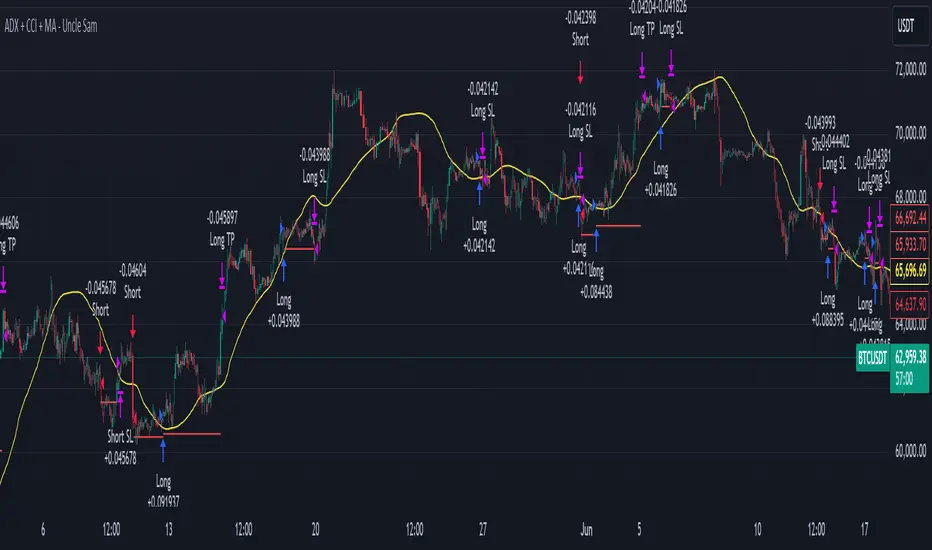
ADX + CCI + MA - Uncle SamStrategy Name: ADX + CCI + MA - Uncle Sam
Overview
This strategy aims to capitalize on trending markets by combining the Average Directional Index (ADX), Commodity Channel Index (CCI), and a customizable Moving Average (MA). It's designed for traders seeking a balanced approach to both long (buy) and short (sell) opportunities. Special thanks to the creators of the ADX and CCI indicators for their invaluable contributions to technical analysis.
Strategy Concept
The core idea is to identify strong trends with the ADX, confirm potential entry points with the CCI, and use the MA to filter trades in the direction of the broader trend. This approach seeks to avoid entering positions during periods of consolidation or when the trend is weak.
Indicator Logic
ADX (Average Directional Index): The ADX measures the strength of a trend, regardless of its direction. A value above the customizable adx_threshold (default 20) signals a strong trend, making it a prime environment for this strategy.
CCI (Commodity Channel Index): The CCI is a momentum oscillator that helps identify overbought (above 100) and oversold (below -100) conditions. We use CCI crossovers to time entries in the direction of the prevailing trend.
MA (Moving Average): The MA acts as a trend filter, ensuring we only enter trades aligned with the overall market direction. You have flexibility in choosing the MA type (SMA, EMA, etc.) and its length to suit your trading style and timeframe.
Entry Conditions
Long (Buy):
ADX is above the adx_threshold.
CCI crosses above 100.
Price is above the chosen Moving Average (if MA trend filtering is enabled).
Short (Sell):
ADX is above the adx_threshold.
CCI crosses below -100.
Price is below the chosen Moving Average (if MA trend filtering is enabled).
Exit Conditions
Stop Loss (SL): Each position has a customizable stop-loss percentage to manage risk. The default setting is 1%.
Take Profit (TP): Each position has a customizable take-profit percentage to secure gains. The default setting is 5%.
MA-Based Risk Management (Optional): This feature allows for early exits if the price closes against the MA trend for a specified number of candles. The default setting is 2 candles.
Default Settings
CCI Period: 15
ADX Length: 10
ADX Threshold: 20
MA Type: HMA
MA Length: 200
MA Source: Close
Commission Fee: $0.0
A commission fee is not added, add your trading/platform commission for realistic trading costs.
Backtest Results
The strategy has been backtested on with the default settings and a starting capital of $1000, with 0.0% commission fee. It shows promising results.
Disclaimer: Backtesting is hypothetical and does not guarantee future performance.
Important Considerations:
Customization: The strategy offers extensive customization to tailor it to your preferences. Experiment with different parameters and settings to find what works best for your trading style.
Risk Management: Always use proper risk management techniques, including position sizing and stop losses, to protect your capital.
MLExtensionsLibrary "MLExtensions"
normalizeDeriv(src, quadraticMeanLength)
Returns the smoothed hyperbolic tangent of the input series.
Parameters:
src : The input series (i.e., the first-order derivative for price).
quadraticMeanLength : The length of the quadratic mean (RMS).
Returns: nDeriv The normalized derivative of the input series.
normalize(src, min, max)
Rescales a source value with an unbounded range to a target range.
Parameters:
src : The input series
min : The minimum value of the unbounded range
max : The maximum value of the unbounded range
Returns: The normalized series
rescale(src, oldMin, oldMax, newMin, newMax)
Rescales a source value with a bounded range to anther bounded range
Parameters:
src : The input series
oldMin : The minimum value of the range to rescale from
oldMax : The maximum value of the range to rescale from
newMin : The minimum value of the range to rescale to
newMax : The maximum value of the range to rescale to
Returns: The rescaled series
color_green(prediction)
Assigns varying shades of the color green based on the KNN classification
Parameters:
prediction : Value (int|float) of the prediction
Returns: color
color_red(prediction)
Assigns varying shades of the color red based on the KNN classification
Parameters:
prediction : Value of the prediction
Returns: color
tanh(src)
Returns the the hyperbolic tangent of the input series. The sigmoid-like hyperbolic tangent function is used to compress the input to a value between -1 and 1.
Parameters:
src : The input series (i.e., the normalized derivative).
Returns: tanh The hyperbolic tangent of the input series.
dualPoleFilter(src, lookback)
Returns the smoothed hyperbolic tangent of the input series.
Parameters:
src : The input series (i.e., the hyperbolic tangent).
lookback : The lookback window for the smoothing.
Returns: filter The smoothed hyperbolic tangent of the input series.
tanhTransform(src, smoothingFrequency, quadraticMeanLength)
Returns the tanh transform of the input series.
Parameters:
src : The input series (i.e., the result of the tanh calculation).
smoothingFrequency
quadraticMeanLength
Returns: signal The smoothed hyperbolic tangent transform of the input series.
n_rsi(src, n1, n2)
Returns the normalized RSI ideal for use in ML algorithms.
Parameters:
src : The input series (i.e., the result of the RSI calculation).
n1 : The length of the RSI.
n2 : The smoothing length of the RSI.
Returns: signal The normalized RSI.
n_cci(src, n1, n2)
Returns the normalized CCI ideal for use in ML algorithms.
Parameters:
src : The input series (i.e., the result of the CCI calculation).
n1 : The length of the CCI.
n2 : The smoothing length of the CCI.
Returns: signal The normalized CCI.
n_wt(src, n1, n2)
Returns the normalized WaveTrend Classic series ideal for use in ML algorithms.
Parameters:
src : The input series (i.e., the result of the WaveTrend Classic calculation).
n1
n2
Returns: signal The normalized WaveTrend Classic series.
n_adx(highSrc, lowSrc, closeSrc, n1)
Returns the normalized ADX ideal for use in ML algorithms.
Parameters:
highSrc : The input series for the high price.
lowSrc : The input series for the low price.
closeSrc : The input series for the close price.
n1 : The length of the ADX.
regime_filter(src, threshold, useRegimeFilter)
Parameters:
src
threshold
useRegimeFilter
filter_adx(src, length, adxThreshold, useAdxFilter)
filter_adx
Parameters:
src : The source series.
length : The length of the ADX.
adxThreshold : The ADX threshold.
useAdxFilter : Whether to use the ADX filter.
Returns: The ADX.
filter_volatility(minLength, maxLength, useVolatilityFilter)
filter_volatility
Parameters:
minLength : The minimum length of the ATR.
maxLength : The maximum length of the ATR.
useVolatilityFilter : Whether to use the volatility filter.
Returns: Boolean indicating whether or not to let the signal pass through the filter.
backtest(high, low, open, startLongTrade, endLongTrade, startShortTrade, endShortTrade, isStopLossHit, maxBarsBackIndex, thisBarIndex)
Performs a basic backtest using the specified parameters and conditions.
Parameters:
high : The input series for the high price.
low : The input series for the low price.
open : The input series for the open price.
startLongTrade : The series of conditions that indicate the start of a long trade.`
endLongTrade : The series of conditions that indicate the end of a long trade.
startShortTrade : The series of conditions that indicate the start of a short trade.
endShortTrade : The series of conditions that indicate the end of a short trade.
isStopLossHit : The stop loss hit indicator.
maxBarsBackIndex : The maximum number of bars to go back in the backtest.
thisBarIndex : The current bar index.
Returns: A tuple containing backtest values
init_table()
init_table()
Returns: tbl The backtest results.
update_table(tbl, tradeStatsHeader, totalTrades, totalWins, totalLosses, winLossRatio, winrate, stopLosses)
update_table(tbl, tradeStats)
Parameters:
tbl : The backtest results table.
tradeStatsHeader : The trade stats header.
totalTrades : The total number of trades.
totalWins : The total number of wins.
totalLosses : The total number of losses.
winLossRatio : The win loss ratio.
winrate : The winrate.
stopLosses : The total number of stop losses.
Returns: Updated backtest results table.

Candles HTF on Heikin Ashi ChartThis script enables calling and/or plotting of traditional Candles sources while loaded on Heikin Ashi charts.
Thanks to @PineCoders for rounding method: www.pinecoders.com
Thanks to @BeeHolder for method to regex normalize syminfo.tickerid.
NOTICE: While this script is meant to be utilized on Heikin Ashi charts it does NOT enable ability to backtest!
NOTICE: For more info on why non standard charts cannot be reliably backtested please see:
NOTICE: This is an example script and not meant to be used as an actual strategy. By using this script or any portion thereof, you acknowledge that you have read and understood that this is for research purposes only and I am not responsible for any financial losses you may incur by using this script!

Trend Following $BTC - Multi-Timeframe Structure + ReversTREND FOLLOWING STRATEGY - MULTI-TIMEFRAME STRUCTURE BREAKOUT SYSTEM
Strategy Overview
This is an enhanced Turtle Trading system designed for cryptocurrency spot trading. It combines Donchian Channel breakouts with multi-timeframe structure filtering and ATR-based dynamic risk management. The strategy trades both long and short positions using reverse signal exits to maximize trend capture.
Core Features
Multi-Timeframe Structure Filtering
The strategy uses Swing High/Low analysis to identify market structure trends. You can customize the structure timeframe (default: 3 minutes) to match your trading style. Only enters trades aligned with the identified trend direction, avoiding counter-trend positions that often lead to losses.
Reverse Signal Exit System
Instead of using fixed stop-losses or time-based exits, this strategy exits positions only when a reverse entry signal triggers. This approach maximizes trend profits and reduces premature exits during normal market retracements.
ATR Dynamic Pyramiding
Automatically adds positions when price moves 0.5 ATR in your favor. Supports up to 2 units maximum (adjustable). This pyramid scaling enhances profitability during strong trends while maintaining disciplined risk management.
Complete Risk Management
Fixed position sizing at 5000 USD per unit. Includes realistic commission fees of 0.06% (Binance spot rate). Initial capital set at 10,000 USD. All backtest parameters reflect real-world trading conditions.
Trading Logic
Entry Conditions
Long Entry: Close price breaks above the 20-period high AND structure trend is bullish (price breaks above Swing High)
Short Entry: Close price breaks below the 20-period low AND structure trend is bearish (price breaks below Swing Low)
Position Scaling
Long positions: Add when price rises 0.5 ATR or more
Short positions: Add when price falls 0.5 ATR or more
Maximum 2 units including initial entry
Exit Conditions
Long Exit: Triggers when short entry signal appears (price breaks 20-period low + structure turns bearish)
Short Exit: Triggers when long entry signal appears (price breaks 20-period high + structure turns bullish)
Default Parameters
Channel Settings
Entry Channel Period: 20 (Donchian Channel breakout period)
Exit Channel Period: 10 (reserved parameter)
ATR Settings
ATR Period: 20
Stop Loss ATR Multiplier: 2.0
Add Position ATR Multiplier: 0.5
Structure Filter
Swing Length: 300 (Swing High/Low calculation period)
Structure Timeframe: 3 minutes
Adjust these based on your trading timeframe and asset volatility
Position Management
Maximum Units: 2 (including initial entry)
Capital Per Unit: 5000 USD
Visualization Features
Background Colors
Light Green: Bullish market structure
Light Red: Bearish market structure
Dark Green: Long position entry
Dark Red: Short position entry
Optional Display Elements (Default: OFF)
Entry and exit channel lines
Structure high/low reference lines
ATR stop-loss indicator
Next position add level
Entry/exit labels
Alert Message Format
The strategy sends notifications with the following format:
Entry: "5m Long EP:90450.50"
Add Position: "15m Add Long 2/2 EP:91000.25"
Exit: "5m Close Long Reverse Signal"
Where the first part shows your current chart timeframe and EP indicates Entry Price
Backtest Settings
Capital Allocation
Initial Capital: 10,000 USD
Per Entry: 5,000 USD (split into 2 potential entries)
Leverage: 0x (spot trading only)
Trading Costs
Commission: 0.06% (Binance spot VIP0 rate)
Slippage: 0 (adjust based on your experience)
Best Use Cases
Ideal Scenarios
Trending markets with clear directional movement
Moderate to high volatility assets
Timeframes from 1-minute to 4-hour charts
Best suited for major cryptocurrencies with good liquidity
Not Recommended For
Highly volatile choppy/ranging markets
Low liquidity small-cap coins
Extreme market conditions or black swan events
Usage Recommendations
Timeframe Guidelines
1-5 minute charts: Use for scalping, consider Swing Length 100-160
15-30 minute charts: Good for short-term trading, Swing Length 50-100
1-4 hour charts: Suitable for swing trading, Swing Length 20-50
Optimization Tips
Always backtest on historical data before live trading
Adjust swing length based on asset volatility and your timeframe
Different cryptocurrencies may require different parameter settings
Enable visualization options initially to understand entry/exit points
Monitor win rate and drawdown during backtesting
Technical Details
Built on Pine Script v6
No repainting - uses proper bar referencing with offset
Prevents lookahead bias with lookahead=off parameter
Strategy mode with accurate commission and slippage modeling
Multi-timeframe security function for structure analysis
Proper position state tracking to avoid duplicate signals
Risk Disclaimer
This strategy is provided for educational and research purposes only. Past performance does not guarantee future results. Backtesting results may differ from live trading due to slippage, execution delays, and changing market conditions. The strategy performs best in trending markets and may experience drawdowns during ranging conditions. Always practice proper risk management and never risk more than you can afford to lose. It is recommended to paper trade first and start with small position sizes when going live.
How to Use
Add the strategy to your TradingView chart
Select your desired timeframe (1m to 4h recommended)
Adjust parameters based on your risk tolerance and trading style
Review backtest results in the Strategy Tester tab
Set up alerts for automated notifications
Consider paper trading before risking real capital
Tags
Trend Following, Turtle Trading, Donchian Channel, Structure Breakout, ATR, Cryptocurrency, Spot Trading, Risk Management, Pyramiding, Multi-Timeframe Analysis
---
Strategy Name: Trend Following BTC
Version: v1.0
Pine Script Version: v6
Last Updated: December 2025

EMA 12-26-100 Momentum Strategy# Triple EMA Multi-Signal Momentum Strategy
## 📊 Overview
**Triple EMA Multi-Signal** is a comprehensive trend-following momentum strategy designed specifically for cryptocurrency markets. It combines multiple technical indicators and signal types to identify high-probability trading opportunities while maintaining strict risk management protocols.
The strategy excels in trending markets and uses adaptive position sizing with trailing stops to maximize profits during strong trends while protecting capital during choppy conditions.
## 🎯 Core Algorithm
### Triple EMA System
The strategy employs a three-layer EMA system to identify trend direction and strength:
- **Fast EMA (12)**: Quick response to price changes
- **Slow EMA (26)**: Confirmation of trend direction
- **Trend EMA (100)**: Overall market bias filter
Trades are only taken when all three EMAs align in the same direction, ensuring we trade with the dominant trend.
### Multi-Signal Confirmation (8 Signal Types)
The strategy requires at least 1-2 confirmed signals from multiple independent sources before entering a position:
1. **EMA Crossover** - Fast EMA crossing Slow EMA (primary signal)
2. **MACD Cross** - MACD line crossing signal line (momentum confirmation)
3. **RSI Reversal** - RSI bouncing from oversold/overbought zones
4. **Price Action** - Strong bullish/bearish candles (>60% of range)
5. **Volume Spike** - Above-average volume confirmation
6. **Breakout** - Price breaking 20-period high/low with volume
7. **Pullback to EMA** - Trend continuation after healthy retracement
8. **Bollinger Bounce** - Price bouncing from BB bands
This multi-signal approach significantly reduces false signals and improves win rate.
## 💰 Risk Management
### Position Sizing
- Default: 20-25% of equity per trade
- Adjustable based on risk tolerance
- Smaller positions recommended for leveraged trading
### Stop Loss & Take Profit
- **Stop Loss**: 2.0% (tight control of risk)
- **Take Profit**: 5.5% (2.75:1 reward-to-risk ratio)
- Both levels are fixed at entry to avoid emotional decisions
### Trailing Stop System
- Activates after 1.8% profit
- Trails at 1.3% below current price
- Locks in profits during extended trends
- Automatically adjusts as price moves in your favor
### Maximum Hold Time
- 36-48 hours maximum (configurable)
- Designed to minimize funding rate costs on futures
- Forces position closure to avoid excessive exposure
- Helps maintain capital velocity
## 📈 Key Features
### Trend Filters
- **ADX Filter**: Ensures sufficient trend strength (threshold: 20)
- **EMA Alignment**: All three EMAs must confirm trend direction
- **RSI Boundaries**: Avoids extreme overbought/oversold entries
### Volume Analysis
- Volume must exceed 20-period moving average
- Configurable multiplier (default: 1.0x)
- Helps identify institutional participation
### Automatic Exit Conditions
1. Take Profit target reached
2. Stop Loss triggered
3. Trailing stop activated
4. Trend reversal (EMA cross in opposite direction)
5. Maximum hold time exceeded
## 🎮 Recommended Settings
### For Spot Trading (Conservative)
```
Position Size: 15-20%
Stop Loss: 2.5%
Take Profit: 6.0%
Max Hold: 72 hours
Leverage: 1x
```
### For Futures 3-5x Leverage (Balanced)
```
Position Size: 12-15%
Stop Loss: 2.0%
Take Profit: 5.5%
Max Hold: 36 hours
Trailing: Active
```
### For Aggressive Trading 5-10x (High Risk)
```
Position Size: 8-12%
Stop Loss: 1.5%
Take Profit: 4.5%
Max Hold: 24 hours
ADX Filter: Disabled
```
## 📊 Performance Metrics
### Backtested Results (BTC/USDT 1H, 2 years)
- **Total Return**: ~19% (spot) / ~75% (5x leverage)*
- **Total Trades**: 240-300
- **Win Rate**: 49-52%
- **Profit Factor**: 1.25-1.50
- **Max Drawdown**: ~18-22%
- **Average Trade**: 0.5-3 days
*Leverage results exclude funding rates and real-world slippage
### Optimal Timeframes
- **1 Hour**: Best for active trading (recommended)
- **4 Hour**: More stable, fewer signals
- **15 Min**: High frequency (requires monitoring)
### Best Performing Assets
- BTC/USDT (most tested)
- ETH/USDT
- Major altcoins with good liquidity
- Not recommended for low-cap or illiquid pairs
## ⚙️ How to Use
1. **Add to Chart**: Apply strategy to 1H BTC/USDT chart
2. **Adjust Settings**: Configure risk parameters based on your preference
3. **Review Signals**: Green = Long, Red = Short, labels show signal count
4. **Monitor Performance**: Check strategy tester for detailed statistics
5. **Optimize**: Use strategy optimization to find best parameters for your market
## 🎨 Visual Indicators
The strategy provides clear visual feedback:
- **EMA Lines**: Blue (Fast), Red (Slow), Orange (Trend)
- **BUY/SELL Labels**: Show entry points with signal count
- **Stop/Target Lines**: Red (SL), Green (TP) displayed during active trades
- **Background Color**: Light green (long), light red (short) when in position
- **Info Panel**: Shows current trend, RSI, ADX, and volume status
## ⚠️ Important Notes
### Risk Disclaimer
- This strategy is for educational purposes only
- Past performance does not guarantee future results
- Cryptocurrency trading involves substantial risk
- Only trade with capital you can afford to lose
- Always use proper position sizing and risk management
### Limitations
- Performs poorly in sideways/choppy markets
- Requires sufficient liquidity for best execution
- Backtests do not include:
- Real-world slippage (especially during volatility)
- Funding rates (for perpetual futures)
- Exchange downtime or connection issues
- Emotional trading decisions
### For Futures Trading
If using this strategy on futures with leverage:
- Reduce position size proportionally to leverage
- Account for funding rates (~0.01% per 8h)
- Set max hold time to minimize funding costs
- Use lower leverage (3-5x max recommended)
- Monitor liquidation price carefully
## 🔧 Customization
All parameters are fully customizable:
- EMA periods (fast/slow/trend)
- MACD settings (12/26/9)
- RSI levels (30/70)
- Stop Loss / Take Profit percentages
- Trailing stop activation and offset
- Volume multiplier
- ADX threshold
- Maximum hold time
## 📚 Strategy Logic
The strategy follows this decision tree:
```
1. Check Trend Direction (EMA alignment)
↓
2. Scan for Entry Signals (8 types)
↓
3. Confirm with Filters (ADX, Volume, RSI)
↓
4. Enter Position with Fixed SL/TP
↓
5. Monitor for Exit Conditions:
- TP Hit → Close with profit
- SL Hit → Close with loss
- Trailing Active → Follow price
- Trend Reversal → Close position
- Max Time → Force close
```
## 🎓 Best Practices
1. **Start Conservative**: Use smaller position sizes initially
2. **Track Performance**: Monitor actual vs backtested results
3. **Optimize Regularly**: Market conditions change, adapt parameters
4. **Combine with Analysis**: Don't rely solely on automated signals
5. **Manage Emotions**: Stick to the system, avoid manual overrides
6. **Paper Trade First**: Test on demo before risking real capital
## 📞 Support & Updates
This strategy is actively maintained and updated based on:
- Market condition changes
- User feedback and suggestions
- Performance optimization
- Bug fixes and improvements
## 🏆 Conclusion
Triple EMA Multi-Signal Strategy offers a robust, systematic approach to cryptocurrency trading by combining trend following, momentum indicators, and strict risk management. Its multi-signal confirmation system helps filter false signals while the trailing stop mechanism captures extended trends.
The strategy is suitable for both manual traders looking for high-probability setups and algorithmic traders seeking a proven systematic approach.
**Remember**: No strategy wins 100% of the time. Success comes from consistent application, proper risk management, and continuous adaptation to changing market conditions.
---
*Version: 1.0*
*Last Updated: November 2025*
*Tested on: BTC/USDT, ETH/USDT (1H, 4H timeframes)*
*Recommended Capital: $5,000+ for optimal position sizing*

Advanced Multi-Timeframe Trading System (Risk Managed)Description:
This strategy is an original approach that combines two main analytical components to identify potential trade opportunities while simulating realistic trading conditions:
1. Market Trend Analysis via an Approximate Hurst Exponent
• What It Does:
The strategy computes a rough measure of market trending using an approximate Hurst exponent. A value above 0.5 suggests persistent, trending behavior, while a value below 0.5 indicates a tendency toward mean-reversion.
• How It’s Used:
The Hurst exponent is calculated on both the chart’s current timeframe and a higher timeframe (default: Daily) to capture both local and broader market dynamics.
2. Fibonacci Retracement Levels
• What It Does:
Using daily high and low data from a selected timeframe (default: Daily), the script computes key Fibonacci retracement levels.
• How It’s Used:
• The 61.8% level (Golden Ratio) serves as a key threshold:
• A long entry is signaled when the price crosses above this level if the daily Hurst exponent confirms a trending market.
• The 38.2% level is used to identify short-entry opportunities when the price crosses below it and the daily Hurst indicates non-trending conditions.
Signal Logic:
• Long Entry:
When the price crosses above the 61.8% Fibonacci level (Golden Ratio) and the daily Hurst exponent is greater than 0.5, suggesting a trending market.
• Short Entry:
When the price crosses below the 38.2% Fibonacci level and the daily Hurst exponent is less than 0.5, indicating a less trending or potentially reversing market.
Risk Management & Trade Execution:
• Stop-Loss:
Each trade is risk-managed with a stop-loss set at 2% below (for longs) or above (for shorts) the entry price. This ensures that no single trade risks more than a small, sustainable portion of the account.
• Take Profit:
A take profit order targets a risk-reward ratio of 1:2 (i.e., the target profit is twice the amount risked).
• Position Sizing:
Trades are executed with a fixed position size equal to 10% of account equity.
• Trade Frequency Limits:
• Daily Limit: A maximum of 5 trades per day
• Overall Limit: No more than 510 trades during the backtesting period (e.g., since 2019)
These limits are imposed to simulate realistic trading frequency and to avoid overtrading in backtest results.
Backtesting Parameters:
• Initial Capital: $10,000
• Commission: 0.1% per trade
• Slippage: 1 tick per bar
These settings aim to reflect the conditions faced by the average trader and help ensure that the backtesting results are realistic and not misleading.
Chart Overlays & Visual Aids:
• Fibonacci Levels:
The key Fibonacci retracement levels are plotted on the chart, and the zone between the 61.8% and 38.2% levels is highlighted to show a key retracement area.
• Market Trend Background:
The chart background is tinted green when the daily Hurst exponent indicates a trending market (value > 0.5) and red otherwise.
• Information Table:
An on-chart table displays key parameters such as the current Hurst exponent, daily Hurst value, the number of trades executed today, and the global trade count.
Disclaimer:
Past performance is not indicative of future results. This strategy is experimental and provided solely for educational purposes. It is essential that you backtest and paper trade using your own settings before considering any live deployment. The Hurst exponent calculation is an approximation and should be interpreted as a rough gauge of market behavior. Adjust the parameters and risk management settings according to your personal risk tolerance and market conditions.
Additional Notes:
• Originality & Usefulness:
This script is an original mashup that combines trend analysis with Fibonacci retracement methods. The description above explains how these components work together to provide trading signals.
• Realistic Results:
The strategy uses realistic account sizes, commission rates, slippage, and risk management rules to generate backtesting results that are representative of real-world trading.
• Educational Purpose:
This script is intended to support the TradingView community by offering insights into combining multiple analysis techniques in one strategy. It is not a “get-rich-quick” system but rather an educational tool to help traders understand risk management and trade signal logic.
By using this script, you acknowledge that trading involves risk and that you are responsible for testing and adjusting the strategy to fit your own trading environment. This publication is fully open source, and any modifications should include proper attribution if significant portions of the code are reused.
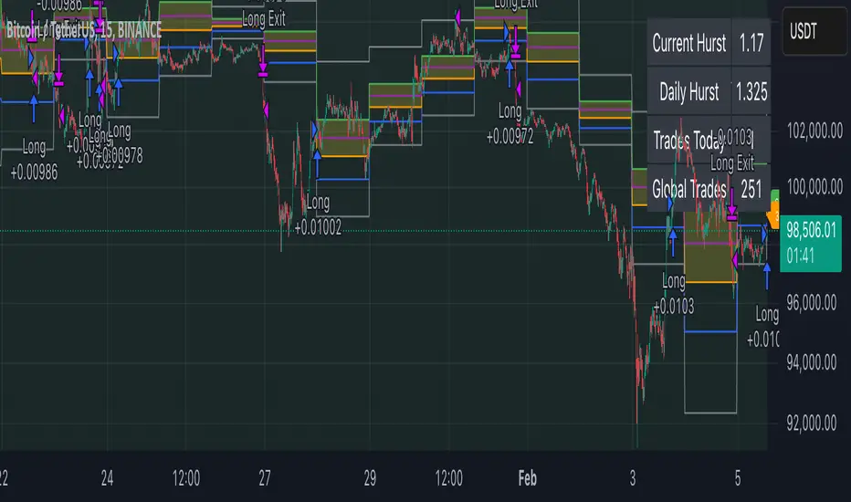
DNSE VN301!, SMA & EMA Cross StrategyDiscover the tailored Pinescript to trade VN30F1M Future Contracts intraday, the strategy focuses on SMA & EMA crosses to identify potential entry/exit points. The script closes all positions by 14:25 to avoid holding any contracts overnight.
HNX:VN301!
www.tradingview.com
Setting & Backtest result:
1-minute chart, initial capital of VND 100 million, entering 4 contracts per time, backtest result from Jan-2024 to Nov-2024 yielded a return over 40%, executed over 1,000 trades (average of 4 trades/day), winning trades rate ~ 30% with a profit factor of 1.10.
The default setting of the script:
A decent optimization is reached when SMA and EMA periods are set to 60 and 15 respectively while the Long/Short stop-loss level is set to 20 ticks (2 points) from the entry price.
Entry & Exit conditions:
Long signals are generated when ema(15) crosses over sma(60) while Short signals happen when ema(15) crosses under sma(60). Long orders are closed when ema(15) crosses under sma(60) while Short orders are closed when ema(15) crosses over sma(60).
Exit conditions happen when (whichever came first):
Another Long/Short signal is generated
The Stop-loss level is reached
The Cut-off time is reached (14:25 every day)
*Disclaimers:
Futures Contracts Trading are subjected to a high degree of risk and price movements can fluctuate significantly. This script functions as a reference source and should be used after users have clearly understood how futures trading works, accessed their risk tolerance level, and are knowledgeable of the functioning logic behind the script.
Users are solely responsible for their investment decisions, and DNSE is not responsible for any potential losses from applying such a strategy to real-life trading activities. Past performance is not indicative/guarantee of future results, kindly reach out to us should you have specific questions about this script.
---------------------------------------------------------------------------------------
Khám phá Pinescript được thiết kế riêng để giao dịch Hợp đồng tương lai VN30F1M trong ngày, chiến lược tập trung vào các đường SMA & EMA cắt nhau để xác định các điểm vào/ra tiềm năng. Chiến lược sẽ đóng tất cả các vị thế trước 14:25 để tránh giữ bất kỳ hợp đồng nào qua đêm.
Thiết lập & Kết quả backtest:
Chart 1 phút, vốn ban đầu là 100 triệu đồng, vào 4 hợp đồng mỗi lần, kết quả backtest từ tháng 1/2024 tới tháng 11/2024 mang lại lợi nhuận trên 40%, thực hiện hơn 1.000 giao dịch (trung bình 4 giao dịch/ngày), tỷ lệ giao dịch thắng ~ 30% với hệ số lợi nhuận là 1,10.
Thiết lập mặc định của chiến lược:
Đạt được một mức tối ưu ổn khi SMA và EMA periods được đặt lần lượt là 60 và 15 trong khi mức cắt lỗ được đặt thành 20 tick (2 điểm) từ giá vào.
Điều kiện Mở và Đóng vị thế:
Tín hiệu Long được tạo ra khi ema(15) cắt trên sma(60) trong khi tín hiệu Short xảy ra khi ema(15) cắt dưới sma(60). Lệnh Long được đóng khi ema(15) cắt dưới sma(60) trong khi lệnh Short được đóng khi ema(15) cắt lên sma(60).
Điều kiện đóng vị thể xảy ra khi (tùy điều kiện nào đến trước):
Một tín hiệu Long/Short khác được tạo ra
Giá chạm mức cắt lỗ
Lệnh chưa đóng nhưng tới giờ cut-off (14:25 hàng ngày)
*Tuyên bố miễn trừ trách nhiệm:
Giao dịch hợp đồng tương lai có mức rủi ro cao và giá có thể dao động đáng kể. Chiến lược này hoạt động như một nguồn tham khảo và nên được sử dụng sau khi người dùng đã hiểu rõ cách thức giao dịch hợp đồng tương lai, đã đánh giá mức độ chấp nhận rủi ro của bản thân và hiểu rõ về logic vận hành của chiến lược này.
Người dùng hoàn toàn chịu trách nhiệm về các quyết định đầu tư của mình và DNSE không chịu trách nhiệm về bất kỳ khoản lỗ tiềm ẩn nào khi áp dụng chiến lược này vào các hoạt động giao dịch thực tế. Hiệu suất trong quá khứ không chỉ ra/cam kết kết quả trong tương lai, vui lòng liên hệ với chúng tôi nếu bạn có thắc mắc cụ thể về chiến lược giao dịch này.
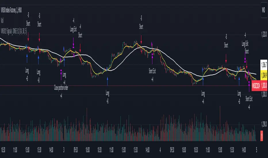
Alans Date Range CalculatorOverview
Setting a date range for backtesting enables you to evaluate your trading strategy under various market conditions. Traders can test a strategy’s performance during specific periods, such as economic downturns, bull markets, or periods of high volatility. This helps assess the trading strategy’s robustness and adaptability across different scenarios.
Specifying years of data instead of just inputting specific start and end dates offers several advantages:
1. **Consistency**: Using a fixed number of years ensures that the testing period is consistent across different strategies or iterations. This makes it easier to compare performance metrics and draw meaningful conclusions.
2. **Flexibility**: Specifying years allows for automatic adjustment of the start date based on the current date or selected end date. This is particularly useful when new data becomes available or when testing on different assets with varying historical data lengths.
3. **Efficiency**: It simplifies updating and retesting strategies. Instead of recalculating specific start dates each time, traders can quickly adjust the number of years to process, making it easier to test strategies over different timeframes.
4. **Comprehensive Analysis**: Broader timeframes defined by years help you evaluate how your strategy performs over multiple market cycles, providing insights into long-term viability and potential weaknesses.
Defining a date range by specifying years allows for more thorough and systematic backtesting, helping traders develop more reliable and effective trading systems.
Alan's Date Range Calculator: A TradingView Pine Script Indicator
Purpose
This Pine Script indicator calculates and displays a date range for backtesting trading strategies. It allows users to specify the number of years to analyze and an end date, then calculates the corresponding start date. Most importantly, users can copy the inputs and function into their own strategies to quickly add a time span feature for backtesting.
Key Features
User-defined input for the number of years to analyze
Customizable end date with a calendar input
Automatic calculation of the start date
Visual display of both start and end dates on the chart
How It Works
User Inputs
Years of Data to Process: An integer input allowing users to specify the number of years for analysis (default: 20, range: 1-100)
End Date: A calendar input for selecting the end date of the analysis period (default: December 31, 2024)
Date Calculation
The script uses a custom function calcStartDate() to determine the start date. It subtracts the specified number of years from the end date's year and sets the start date to January 1st of that year.
Visual Output
The indicator displays two labels on the chart:
Start Date Label: Shows the calculated start date
End Date Label: Displays the user-specified end date
Both labels are positioned horizontally at the bottom of the chart, with the end date label to the right of the start date label.
Applications
This indicator is particularly useful for traders who want to:
Define specific date ranges for backtesting strategies
Quickly visualize the time span of their analysis
Ensure consistent testing periods across different strategies or assets
Customization
Users can easily adjust the analysis period by changing the number of years or selecting a different end date. This flexibility allows for testing strategies across various market conditions and time frames.

Hyperbolic Tangent Volatility Stop [InvestorUnknown]The Hyperbolic Tangent Volatility Stop (HTVS) is an advanced technical analysis tool that combines the smoothing capabilities of the Hyperbolic Tangent Moving Average (HTMA) with a volatility-based stop mechanism. This indicator is designed to identify trends and reversals while accounting for market volatility.
Hyperbolic Tangent Moving Average (HTMA):
The HTMA is at the heart of the HTVS. This custom moving average uses a hyperbolic tangent transformation to smooth out price fluctuations, focusing on significant trends while ignoring minor noise. The transformation reduces the sensitivity to sharp price movements, providing a clearer view of the underlying market direction.
The hyperbolic tangent function (tanh) is commonly used in mathematical fields like calculus, machine learning and signal processing due to its properties of “squashing” inputs into a range between -1 and 1. The function provides a non-linear transformation that can reduce the impact of extreme values while retaining a certain level of smoothness.
tanh(x) =>
e_x = math.exp(x)
e_neg_x = math.exp(-x)
(e_x - e_neg_x) / (e_x + e_neg_x)
The HTMA is calculated by applying a non-linear transformation to the difference between the source price and its simple moving average, then adjusting it using the standard deviation of the price data. The result is a moving average that better tracks the real market direction.
htma(src, len, mul) =>
tanh_src = tanh((src - ta.sma(src, len)) * mul) * ta.stdev(src, len) + ta.sma(src, len)
htma = ta.sma(tanh_src, len)
Important Note: The Hyperbolic Tangent function becomes less accurate with very high prices. For assets priced above 100,000, the results may deteriorate, and for prices exceeding 1 million, the function may stop functioning properly. Therefore, this indicator is better suited for assets with lower prices or lower price ratios.
Volatility Stop (VolStop):
HTVS employs a Volatility Stop mechanism based on the Average True Range (ATR). This stop dynamically adjusts based on market volatility, ensuring that the indicator adapts to changing conditions and avoids false signals in choppy markets.
The VolStop follows the price, with a higher ATR pushing the stop farther away to avoid premature exits during volatile periods. Conversely, when volatility is low, the stop tightens to lock in profits as the trend progresses.
The ATR Length and ATR Multiplier are customizable, allowing traders to control how tightly or loosely the stop follows the price.
pine_volStop(src, atrlen, atrfactor) =>
if not na(src)
var max = src
var min = src
var uptrend = true
var float stop = na
atrM = nz(ta.atr(atrlen) * atrfactor, ta.tr)
max := math.max(max, src)
min := math.min(min, src)
stop := nz(uptrend ? math.max(stop, max - atrM) : math.min(stop, min + atrM), src)
uptrend := src - stop >= 0.0
if uptrend != nz(uptrend , true)
max := src
min := src
stop := uptrend ? max - atrM : min + atrM
Backtest Mode:
HTVS includes a built-in backtest mode, allowing traders to evaluate the indicator's performance on historical data. In backtest mode, it calculates the cumulative equity curve and compares it to a simple buy and hold strategy.
Backtesting features can be adjusted to focus on specific signal types, such as Long Only, Short Only, or Long & Short.
An optional Buy and Hold Equity plot provides insight into how the indicator performs relative to simply holding the asset over time.
The indicator includes a Hints Table, which provides useful recommendations on how to best display the indicator for different use cases. For example, when using the overlay mode, it suggests displaying the indicator in the same pane as price action, while backtest mode is recommended to be used in a separate pane for better clarity.
The Hyperbolic Tangent Volatility Stop offers traders a balanced approach to trend-following, using the robustness of the HTMA for smoothing and the adaptability of the Volatility Stop to avoid whipsaw trades during volatile periods. With its backtesting features and alert system, this indicator provides a comprehensive toolkit for active traders.
RSI SMA Crossover StrategyOverview
RSI SMA Crossover Strategy works the same way as traditional MA crossover strategies, but using RSI instead of price. When RSI crosses over the SMA, a long position is opened (buy). When RSI crosses under the SMA, the long position is closed (sell).
This strategy can be very effective when the right inputs are used (see below). Be sure to use the backtesting tool to determine the optimal parameters for a given asset/timeframe.
Inputs/Parameters
RSI Length: length for RSI calculation (default = 50)
SMA Length: length for SMA calculation (default = 25)
Strategy Properties
Initial Capital = $1000
No default properties are defined for Slippage, Commission, etc, so be sure to set these values to get accurate backtesting results. This script is being published open-source for a reason - save yourself a copy and adjust the settings as you like!
Backtesting Results
Testing on Bitcoin (all time index) 1D chart, with all default parameters.
$1,000 initial investment on 10/07/2010 turns into almost $2.5 billion as of 08/30/2022 (compared to $334 million if the initial investment was held over the same period)
Remember, results can vary greatly based on the variables mentioned above, so always be sure to backtest.
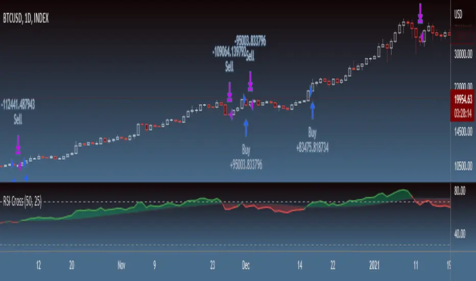
Stochastic Pop and Drop by Jake Bernstein v1 [Bitduke]I found a simple strategy by Jake Bernstein, modified it a little and created a strategy with Risk Management System (SL+TP); After that I test it on the different cryptocurrency pairs.
About the Indicator
Basically it's the strategy of 2 indicators: Stochastic Oscillator to define the bias and Average Directional Index to confirm it.
One again, It uses Stochastic Oscillator to define the trading bias. In particular, the trading bias was deemed bullish when the weekly 14-period Stochastic Oscillator was above some default value (in him paper - 50) and rising and vice versa.
Once the trading bias is established, Steckler used the Average Directional Index (ADX) to define a slowdown in the trend. ADX measures the strength of the trend and a move below 20 signals a weak trend.
Modifications
I didn't implement Average Directional Index (ADX) and test just different sources for data, oscillator periods and different levels in relation to the crypto market.
So, it shows good results with two tight thresholds at 55 and 45 level.
The bar chart below the defining the bullish and bearish periods (green and red) and gives a signal to enter the trade (purple bars).
Backtesting
Backtested on XBTUSD , BTCPERP (FTX) pairs. You may notice it shows good results on 3h timeframe.
Relatively low drawdown
~ 10% (from 2019 to date) FTX
~ 22% (4 years from 2016) Bitmex
I backtested on the different altcoin pairs as well, but the results were just not good.
Relatively good results were shown by some index pairs from the FTX exchange ( FTX:SHITPERP ), but I think there is a few data for backtesting to be asure in them.
Bitmex 3h (2017 - 2020) :
i.imgur.com
FTX 3h (2019 - 2020):
i.imgur.com
Possible Improvements
- Regarding trading algorithm it would be good to check with strategy with ADX somehow. Maybe for the better entries
- As for Risk Management system, it can be improved by adding trailing stop to the strategy.
Link: school.stockcharts.com

Super Trend Daily 2.0 Alerts BFThis is an alerts script for my Super Trend 2.0 indicator . It is intended as a companion script so you can backtest using the Strategy script and generate alerts using this Study script.
This Study script has the same default settings as the Strategy script and its only purpose is to provide alerts for the long and short signals the Strategy generates. Obviously, if you want to generate alerts based on a Strategy backtest, please ensure the settings are the same in the Study as in the Strategy.
For illustration, I have plotted arrows on the chart for long and short signals, and also colored the background to show when the rate of change function determines a choppy/sideways market.
ALERTS
There are 2 alerts set up:
Long Entry
Short Entry
ILLUSTRATION
Green arrow = Long Entry
Red arrow = Short Entry
White background = No short trades
Aqua background = No long trades
EXAMPLE USE CASE
1. Open a Bitcoin/USD chart on 1D timeframe.
2. Open this script and the Super Trend 2.0 indicator script.
3. Backtest with the Strategy Backtester and change the settings if you like until you get a desirable outcome for your own purposes.
4. Once you are happy with the backtest, change the settings in the Alerts script (this one) so they match the Strategy settings.
5. Set up the alerts according to your preferences.
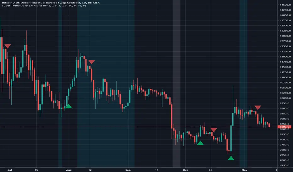
Advanced ICC Multi-Timeframe 1.0Advanced ICC Multi-Timeframe Trading System
A comprehensive implementation and interpretation of the Indication, Correction, Continuation (ICC) trading methodology made popular by Trades by Sci, enhanced with advanced multi-timeframe analysis and automation features.
⚠️ CRITICAL TRADING WARNINGS:
DO NOT blindly follow BUY/SELL signals from this indicator
This indicator shows potential entry points but YOU must validate each trade
PAPER TRADE EXTENSIVELY before risking real capital
BACKTEST THOROUGHLY on your chosen instruments and timeframes
The ICC methodology requires understanding and discretion - automated signals are guidance only
This tool aids analysis but does not replace proper trade planning, risk management, or trader judgment
⚠️ Important Disclaimers:
This indicator is not endorsed by or affiliated with Trades by Sci
This is an early implementation and interpretation of the ICC methodology
May not work exactly as Trades by Sci executes his trades and entries
Requires further debugging, backtesting, and real-world validation
Completely free to use - no purchase required
I'm just one person obsessed with this method and wanted some better visualization of the chart/entries
About ICC:
The ICC method identifies complete market cycles through three phases: Indication (breakout), Correction (pullback), and Continuation (entry). This indicator automates the identification of these phases and adds powerful features for modern traders.
Key Features:
Multi-Timeframe Capabilities:
Automatic timeframe detection with optimized settings for 5m, 15m, 30m, 1H, 4H, and Daily charts
Higher timeframe overlay to view HTF ICC levels on lower timeframe charts for precise entry timing
Smart defaults that adjust swing length and consolidation detection based on your timeframe
Advanced Phase Tracking:
Complete ICC cycle tracking: Indication, Correction, Consolidation, Continuation, and No Setup phases
Live structure detection shows potential peaks/troughs before full confirmation
Intelligent invalidation logic detects failed setups when market structure reverses
Dynamic phase backgrounds for instant visual confirmation
Three Types of Entry Signals:
Traditional Entries - Price crosses back through the original indication level (strongest signals)
"BUY" (green) / "SELL" (red)
Breakout Entries - Price breaks out of consolidation range in the same direction
"BUY" (green) / "SELL" (red)
Reversal Entries (Optional, can be toggled off) - Price breaks consolidation in opposite direction, indicating failed setup
"⚠ BUY" (yellow) / "⚠ SELL" (orange)
More aggressive, counter-trend signals
Can be disabled for more conservative trading
Professional Features:
Volatility-based support/resistance zones (ATR-adjusted) that adapt to market conditions
Historical zone tracking (0-3 configurable) with visual hierarchy
Comprehensive real-time info table displaying all key metrics
Full alert system for entries, indications, and consolidation detection
Visual distinction between high-confidence trend entries and cautionary reversal entries
📖 USAGE GUIDE
Entry Signal Types:
The indicator provides three types of entry signals with visual distinction:
Strong Entries (High Confidence):
"BUY" (bright green) / "SELL" (bright red)
Includes traditional entries (crossing back through indication level) and breakout entries (breaking consolidation in trend direction)
These are trend continuation or breakout signals with higher probability
Recommended for all traders
Reversal Entries (Caution - Counter-Trend):
"⚠ BUY" (yellow) / "⚠ SELL" (orange)
Triggered when price breaks out of correction/consolidation in the OPPOSITE direction
Indicates a failed setup and potential trend reversal
More aggressive, counter-trend plays
Can be toggled off in settings for more conservative trading
Recommended only for experienced traders or after thorough backtesting
Swing Length Settings:
The swing length determines how many bars on each side are needed to confirm a swing high/low. This is the most important setting for tuning the indicator to your style.
Auto Mode (Recommended for beginners): Toggle "Use Auto Timeframe Settings" ON
5-minute: 30 bars
15-minute: 20 bars
30-minute: 12 bars
1-hour: 7 bars
4-hour: 5 bars
Daily: 3 bars
Manual Mode: Toggle "Use Auto Timeframe Settings" OFF
Lower values (3-7): More aggressive, detects smaller swings
Pros: More signals, faster entries, catches smaller moves
Cons: More noise, more false signals, requires tighter stops
Best for: Scalping, active day trading, volatile markets
Higher values (12-20): More conservative, only major swings
Pros: More reliable signals, fewer false breakouts, clearer structure
Cons: Fewer signals, delayed entries, might miss smaller opportunities
Best for: Swing trading, position trading, trending markets
Default Manual Setting: 7 bars (balanced for 1H charts)
Minimum: 3 bars
Consolidation Bars Setting:
Determines how many bars without new structure are needed before flagging consolidation.
Lower values (3-10): Faster detection, catches brief pauses, more sensitive
Best for: Lower timeframes, volatile markets, avoiding any chop
Higher values (20-40): More reliable, only flags true extended consolidation
Best for: Higher timeframes, trending markets, patient traders
Current defaults scale with timeframe (more bars needed on shorter timeframes)
Historical S/R Zones:
Shows previous support and resistance levels to provide context.
Default: 2 historical zones (shows current + 2 previous)
Range: 0-3 zones
Visual Hierarchy: Older zones are more transparent with dashed borders
Usage: Higher numbers (2-3) show more historical context but can clutter the chart. Start with 2 and adjust based on your preference.
Live Structure Feature (Yellow Warning ⚠):
Provides early warning of potential structure changes before full confirmation.
What it does: Detects potential swing highs/lows after just 2 bars instead of waiting for full swing_length confirmation
Live Peak: Shows when a high is followed by 2 lower closes (potential top forming)
Live Trough: Shows when a low is followed by 2 higher closes (potential bottom forming)
Important: These are UNCONFIRMED - they may be invalidated if price reverses
Use case: Get early awareness of potential reversals while waiting for confirmation
Displayed in: Info table only (no visual markers on chart to reduce clutter)
Only shows: Peaks higher than last swing high, or troughs lower than last swing low (filters out noise)
Higher Timeframe (HTF) Analysis:
View higher timeframe ICC structure while trading on lower timeframes.
How to enable: Toggle "Show Higher Timeframe ICC" ON
Setup: Set "Higher Timeframe" to your reference timeframe
Example: Trading on 15-minute? Set HTF to 240 (4-hour) or 60 (1-hour)
Example: Trading on 5-minute? Set HTF to 60 (1-hour) or 15 (15-minute)
What it shows:
HTF indication levels displayed as dashed lines
Blue = HTF Bullish Indication
Purple = HTF Bearish Indication
HTF phase and levels shown in info table
Trading workflow:
Check HTF phase for overall market direction
Wait for HTF correction phase
Drop to lower timeframe to find precise entries
Enter when lower TF shows continuation in alignment with HTF
Best practice: HTF should be 3-4x your trading timeframe for best results
Reversal Entries Toggle:
Default: ON (shows all signal types)
Toggle OFF for more conservative trading (only trend continuation signals)
Recommended: Backtest with both settings to see which works better for your style
New traders should consider disabling reversal entries initially
Volatility-Based Zones:
When enabled, support/resistance zones automatically adjust their height based on ATR (Average True Range).
More volatile = wider zones
Less volatile = tighter zones
Toggle OFF for fixed-width zones
Community Feedback Welcome:
This is an evolving project and your input is valuable! Please share:
Bug reports and issues you encounter
Feature requests and suggestions for improvement
Results from your backtesting and live trading experience
Feedback on the reversal entry feature (too aggressive? working well?)
Ideas for better aligning with the ICC methodology
Perfect for traders learning or implementing the ICC methodology with the benefit of modern automation, multi-timeframe analysis, and flexible entry signal options.

Volatility-Targeted Momentum Portfolio [BackQuant]Volatility-Targeted Momentum Portfolio
A complete momentum portfolio engine that ranks assets, targets a user-defined volatility, builds long, short, or delta-neutral books, and reports performance with metrics, attribution, Monte Carlo scenarios, allocation pie, and efficiency scatter plots. This description explains the theory and the mechanics so you can configure, validate, and deploy it with intent.
Table of contents
What the script does at a glance
Momentum, what it is, how to know if it is present
Volatility targeting, why and how it is done here
Portfolio construction modes: Long Only, Short Only, Delta Neutral
Regime filter and when the strategy goes to cash
Transaction cost modelling in this script
Backtest metrics and definitions
Performance attribution chart
Monte Carlo simulation
Scatter plot analysis modes
Asset allocation pie chart
Inputs, presets, and deployment checklist
Suggested workflow
1) What the script does at a glance
Pulls a list of up to 15 tickers, computes a simple momentum score on each over a configurable lookback, then volatility-scales their bar-to-bar return stream to a target annualized volatility.
Ranks assets by raw momentum, selects the top 3 and bottom 3, builds positions according to the chosen mode, and gates exposure with a fast regime filter.
Accumulates a portfolio equity curve with risk and performance metrics, optional benchmark buy-and-hold for comparison, and a full alert suite.
Adds visual diagnostics: performance attribution bars, Monte Carlo forward paths, an allocation pie, and scatter plots for risk-return and factor views.
2) Momentum: definition, detection, and validation
Momentum is the tendency of assets that have performed well to continue to perform well, and of underperformers to continue underperforming, over a specific horizon. You operationalize it by selecting a horizon, defining a signal, ranking assets, and trading the leaders versus laggards subject to risk constraints.
Signal choices . Common signals include cumulative return over a lookback window, regression slope on log-price, or normalized rate-of-change. This script uses cumulative return over lookback bars for ranking (variable cr = price/price - 1). It keeps the ranking simple and lets volatility targeting handle risk normalization.
How to know momentum is present .
Leaders and laggards persist across adjacent windows rather than flipping every bar.
Spread between average momentum of leaders and laggards is materially positive in sample.
Cross-sectional dispersion is non-trivial. If everything is flat or highly correlated with no separation, momentum selection will be weak.
Your validation should include a diagnostic that measures whether returns are explained by a momentum regression on the timeseries.
Recommended diagnostic tool . Before running any momentum portfolio, verify that a timeseries exhibits stable directional drift. Use this indicator as a pre-check: It fits a regression to price, exposes slope and goodness-of-fit style context, and helps confirm if there is usable momentum before you force a ranking into a flat regime.
3) Volatility targeting: purpose and implementation here
Purpose . Volatility targeting seeks a more stable risk footprint. High-vol assets get sized down, low-vol assets get sized up, so each contributes more evenly to total risk.
Computation in this script (per asset, rolling):
Return series ret = log(price/price ).
Annualized volatility estimate vol = stdev(ret, lookback) * sqrt(tradingdays).
Leverage multiplier volMult = clamp(targetVol / vol, 0.1, 5.0).
This caps sizing so extremely low-vol assets don’t explode weight and extremely high-vol assets don’t go to zero.
Scaled return stream sr = ret * volMult. This is the per-bar, risk-adjusted building block used in the portfolio combinations.
Interpretation . You are not levering your account on the exchange, you are rescaling the contribution each asset’s daily move has on the modeled equity. In live trading you would reflect this with position sizing or notional exposure.
4) Portfolio construction modes
Cross-sectional ranking . Assets are sorted by cr over the chosen lookback. Top and bottom indices are extracted without ties.
Long Only . Averages the volatility-scaled returns of the top 3 assets: avgRet = mean(sr_top1, sr_top2, sr_top3). Position table shows per-asset leverages and weights proportional to their current volMult.
Short Only . Averages the negative of the volatility-scaled returns of the bottom 3: avgRet = mean(-sr_bot1, -sr_bot2, -sr_bot3). Position table shows short legs.
Delta Neutral . Long the top 3 and short the bottom 3 in equal book sizes. Each side is sized to 50 percent notional internally, with weights within each side proportional to volMult. The return stream mixes the two sides: avgRet = mean(sr_top1,sr_top2,sr_top3, -sr_bot1,-sr_bot2,-sr_bot3).
Notes .
The selection metric is raw momentum, the execution stream is volatility-scaled returns. This separation is deliberate. It avoids letting volatility dominate ranking while still enforcing risk parity at the return contribution stage.
If everything rallies together and dispersion collapses, Long Only may behave like a single beta. Delta Neutral is designed to extract cross-sectional momentum with low net beta.
5) Regime filter
A fast EMA(12) vs EMA(21) filter gates exposure.
Long Only active when EMA12 > EMA21. Otherwise the book is set to cash.
Short Only active when EMA12 < EMA21. Otherwise cash.
Delta Neutral is always active.
This prevents taking long momentum entries during obvious local downtrends and vice versa for shorts. When the filter is false, equity is held flat for that bar.
6) Transaction cost modelling
There are two cost touchpoints in the script.
Per-bar drag . When the regime filter is active, the per-bar return is reduced by fee_rate * avgRet inside netRet = avgRet - (fee_rate * avgRet). This models proportional friction relative to traded impact on that bar.
Turnover-linked fee . The script tracks changes in membership of the top and bottom baskets (top1..top3, bot1..bot3). The intent is to charge fees when composition changes. The template counts changes and scales a fee by change count divided by 6 for the six slots.
Use case: increase fee_rate to reflect taker fees and slippage if you rebalance every bar or trade illiquid assets. Reduce it if you rebalance less often or use maker orders.
Practical advice .
If you rebalance daily, start with 5–20 bps round-trip per switch on liquid futures and adjust per venue.
For crypto perp microcaps, stress higher cost assumptions and add slippage buffers.
If you only rotate on lookback boundaries or at signals, use alert-driven rebalances and lower per-bar drag.
7) Backtest metrics and definitions
The script computes a standard set of portfolio statistics once the start date is reached.
Net Profit percent over the full test.
Max Drawdown percent, tracked from running peaks.
Annualized Mean and Stdev using the chosen trading day count.
Variance is the square of annualized stdev.
Sharpe uses daily mean adjusted by risk-free rate and annualized.
Sortino uses downside stdev only.
Omega ratio of sum of gains to sum of losses.
Gain-to-Pain total gains divided by total losses absolute.
CAGR compounded annual growth from start date to now.
Alpha, Beta versus a user-selected benchmark. Beta from covariance of daily returns, Alpha from CAPM.
Skewness of daily returns.
VaR 95 linear-interpolated 5th percentile of daily returns.
CVaR average of the worst 5 percent of daily returns.
Benchmark Buy-and-Hold equity path for comparison.
8) Performance attribution
Cumulative contribution per asset, adjusted for whether it was held long or short and for its volatility multiplier, aggregated across the backtest. You can filter to winners only or show both sides. The panel is sorted by contribution and includes percent labels.
9) Monte Carlo simulation
The panel draws forward equity paths from either a Normal model parameterized by recent mean and stdev, or non-parametric bootstrap of recent daily returns. You control the sample length, number of simulations, forecast horizon, visibility of individual paths, confidence bands, and a reproducible seed.
Normal uses Box-Muller with your seed. Good for quick, smooth envelopes.
Bootstrap resamples realized returns, preserving fat tails and volatility clustering better than a Gaussian assumption.
Bands show 10th, 25th, 75th, 90th percentiles and the path mean.
10) Scatter plot analysis
Four point-cloud modes, each plotting all assets and a star for the current portfolio position, with quadrant guides and labels.
Risk-Return Efficiency . X is risk proxy from leverage, Y is expected return from annualized momentum. The star shows the current book’s composite.
Momentum vs Volatility . Visualizes whether leaders are also high vol, a cue for turnover and cost expectations.
Beta vs Alpha . X is a beta proxy, Y is risk-adjusted excess return proxy. Useful to see if leaders are just beta.
Leverage vs Momentum . X is volMult, Y is momentum. Shows how volatility targeting is redistributing risk.
11) Asset allocation pie chart
Builds a wheel of current allocations.
Long Only, weights are proportional to each long asset’s current volMult and sum to 100 percent.
Short Only, weights show the short book as positive slices that sum to 100 percent.
Delta Neutral, 50 percent long and 50 percent short books, each side leverage-proportional.
Labels can show asset, percent, and current leverage.
12) Inputs and quick presets
Core
Portfolio Strategy . Long Only, Short Only, Delta Neutral.
Initial Capital . For equity scaling in the panel.
Trading Days/Year . 252 for stocks, 365 for crypto.
Target Volatility . Annualized, drives volMult.
Transaction Fees . Per-bar drag and composition change penalty, see the modelling notes above.
Momentum Lookback . Ranking horizon. Shorter is more reactive, longer is steadier.
Start Date . Ensure every symbol has data back to this date to avoid bias.
Benchmark . Used for alpha, beta, and B&H line.
Diagnostics
Metrics, Equity, B&H, Curve labels, Daily return line, Rolling drawdown fill.
Attribution panel. Toggle winners only to focus on what matters.
Monte Carlo mode with Normal or Bootstrap and confidence bands.
Scatter plot type and styling, labels, and portfolio star.
Pie chart and labels for current allocation.
Presets
Crypto Daily, Long Only . Lookback 25, Target Vol 50 percent, Fees 10 bps, Regime filter on, Metrics and Drawdown on. Monte Carlo Bootstrap with Recent 200 bars for bands.
Crypto Daily, Delta Neutral . Lookback 25, Target Vol 50 percent, Fees 15–25 bps, Regime filter always active for this mode. Use Scatter Risk-Return to monitor efficiency and keep the star near upper left quadrants without drifting rightward.
Equities Daily, Long Only . Lookback 60–120, Target Vol 15–20 percent, Fees 5–10 bps, Regime filter on. Use Benchmark SPX and watch Alpha and Beta to keep the book from becoming index beta.
13) Suggested workflow
Universe sanity check . Pick liquid tickers with stable data. Thin assets distort vol estimates and fees.
Check momentum existence . Run on your timeframe. If slope and fit are weak, widen lookback or avoid that asset or timeframe.
Set risk budget . Choose a target volatility that matches your drawdown tolerance. Higher target increases turnover and cost sensitivity.
Pick mode . Long Only for bull regimes, Short Only for sustained downtrends, Delta Neutral for cross-sectional harvesting when index direction is unclear.
Tune lookback . If leaders rotate too often, lengthen it. If entries lag, shorten it.
Validate cost assumptions . Increase fee_rate and stress Monte Carlo. If the edge vanishes with modest friction, refine selection or lengthen rebalance cadence.
Run attribution . Confirm the strategy’s winners align with intuition and not one unstable outlier.
Use alerts . Enable position change, drawdown, volatility breach, regime, momentum shift, and crash alerts to supervise live runs.
Important implementation details mapped to code
Momentum measure . cr = price / price - 1 per symbol for ranking. Simplicity helps avoid overfitting.
Volatility targeting . vol = stdev(log returns, lookback) * sqrt(tradingdays), volMult = clamp(targetVol / vol, 0.1, 5), sr = ret * volMult.
Selection . Extract indices for top1..top3 and bot1..bot3. The arrays rets, scRets, lev_vals, and ticks_arr track momentum, scaled returns, leverage multipliers, and display tickers respectively.
Regime filter . EMA12 vs EMA21 switch determines if the strategy takes risk for Long or Short modes. Delta Neutral ignores the gate.
Equity update . Equity multiplies by 1 + netRet only when the regime was active in the prior bar. Buy-and-hold benchmark is computed separately for comparison.
Tables . Position tables show current top or bottom assets with leverage and weights. Metric table prints all risk and performance figures.
Visualization panels . Attribution, Monte Carlo, scatter, and pie use the last bars to draw overlays that update as the backtest proceeds.
Final notes
Momentum is a portfolio effect. The edge comes from cross-sectional dispersion, adequate risk normalization, and disciplined turnover control, not from a single best asset call.
Volatility targeting stabilizes path but does not fix selection. Use the momentum regression link above to confirm structure exists before you size into it.
Always test higher lag costs and slippage, then recheck metrics, attribution, and Monte Carlo envelopes. If the edge persists under stress, you have something robust.
