BAS EnhancedBAS Enhanced Indicator – A Powerful Market Trend & Volatility Tool
The BAS Enhanced Indicator is a cutting-edge trading tool designed to help traders analyze market trends, volatility, and price momentum with precision. This indicator builds upon traditional Bollinger Bands concepts, integrating adaptive price action tracking, dynamic band width analysis, and advanced smoothing techniques to generate clear and actionable trading insights.
🔹 Key Features & Benefits:
✅ Smart Price Selection – Choose between Close, High, Low, HL2, or HLC3 to tailor the indicator to different market conditions.
✅ Dynamic Band Analysis – Measures price movements relative to dynamically calculated upper and lower bands for real-time market assessment.
✅ Volatility & Trend Strength Measurement – The indicator uses a unique Width Calculation (wd) to gauge market volatility, helping traders understand the strength of price movements.
✅ Composite Indicator Calculation – Combines price position and band width with customizable power functions to provide a more refined momentum signal.
✅ Smoothing for Accuracy – Uses Exponential Moving Average (EMA) and Simple Moving Average (SMA) for a clearer trend visualization, reducing noise in volatile markets.
✅ Two Signal Lines for Confirmation – Includes customizable bullish and bearish signal lines, allowing traders to identify breakouts and reversals with greater confidence.
✅ Visual & Alert-Based Trading Signals – The indicator plots:
Smoothed Composite Indicator (Blue Line) – Tracks market momentum
%D Moving Average (Red Line) – A secondary smoothing layer for trend confirmation
Mid Values (Orange & Purple Lines) – Additional volatility references
Signal Lines (Green & Red Horizontal Lines) – Key breakout levels
✅ Built-in Alerts for Trade Signals – Get notified instantly when:
Bullish Alert 🚀 – The indicator crosses above the upper signal line
Bearish Alert 📉 – The indicator crosses below the lower signal line
📈 How to Use the BAS Enhanced Indicator?
🔹 Trend Trading: Use crossovers above Signal Line 2 as a potential buy signal and crossovers below Signal Line 1 as a potential sell signal.
🔹 Volatility Monitoring: When the band width (wd) expands, market volatility is increasing – ideal for breakout traders. When wd contracts, market volatility is low, signaling potential consolidation.
🔹 Momentum Confirmation: Use the %D Moving Average to confirm sustained trend movements before entering a trade.
🚀 Why Use BAS Enhanced?
This indicator is perfect for day traders, swing traders, and trend-followers looking to enhance their market timing, filter false signals, and improve decision-making. Whether you're trading stocks, forex, or crypto, BAS Enhanced helps you stay ahead of market movements with precision and clarity.
🔔 Add BAS Enhanced to your TradingView toolkit today and trade smarter with confidence!
ابحث في النصوص البرمجية عن "band"

Margen de confianzaIt uses two moving averages (20 and 80). Based on their crossovers, you draw parallel bands.
The zone between these bands signals “confidence.” A downside break warns of risk; an upside break suggests price could push to new highs.
Son 2 medias moviles. Una de 20 y otra de 80. Utilizando los cruces se puede trazar lineas paralelas.
En las zonas que quedan entre estas lineas hay "confianza". Si el precio atraviesa para abajo hay peligro y si atraviesa para arriba puede ir a romper maximos

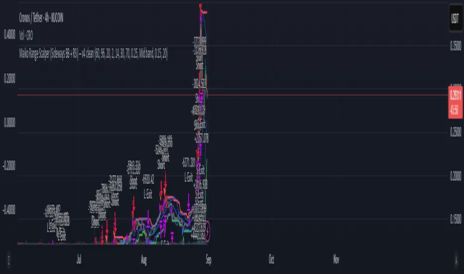
Maiko Range Scalper (Sideways BB + RSI) – v4 cleanPurpose
It’s a range scalping strategy for crypto. It tries to take small, repeatable trades inside a sideways market: buy near the bottom of the range, sell near the middle/top (and the reverse for shorts).
Core idea (two timeframes)
Define the trading range on a higher timeframe (HTF)
You choose the HTF (e.g., 15m or 1h).
The script finds the highest high and lowest low over a lookback window (e.g., last 96 HTF candles) → these become HTF Resistance and HTF Support.
It also calculates the midline (average of support/resistance).
Trade signals on your lower timeframe (LTF)
You run the strategy on a fast chart (e.g., 1m or 5m).
Entries are only allowed inside the HTF range.
Entry logic (mean reversion)
Indicators on the LTF:
Bollinger Bands (length & std dev configurable).
RSI (length & thresholds configurable).
Optional VWAP proximity filter (price must be within X% of VWAP).
Long setup:
Price touches/under-cuts the lower Bollinger band AND RSI ≤ threshold (default 30) AND price is inside the HTF range (and passes VWAP filter if enabled).
Short setup:
Price touches/exceeds the upper Bollinger band AND RSI ≥ threshold (default 70) AND price is inside the HTF range (and passes VWAP filter if enabled).
Exits and risk
Stop-loss: placed just outside the HTF range with a configurable buffer %:
Long SL = HTF Support × (1 − buffer).
Short SL = HTF Resistance × (1 + buffer).
Take-profit (selectable):
Mid band (the Bollinger basis) → conservative, faster exits.
Opposite band / HTF boundary → more aggressive, higher RR but more give-backs.
Position sizing
A simple cap: maximum position size = percent of account equity (e.g., 20%).
The script calculates quantity from that cap and current price.
Plots you’ll see on the chart
HTF Resistance (red) and HTF Support (green) via plot().
HTF Midline (gray dashed) drawn with a line.new() object (because plot() cannot do dashed).
Bollinger basis/upper/lower on the LTF.
Optional VWAP line (only shown if you enable the filter).
Signal markers (green triangle up for Long setups, red triangle down for Short setups).
Alerts
Two alertconditions:
“Long Setup” – when a long entry condition appears.
“Short Setup” – when a short entry condition appears.
Create alerts from these to get notified in real time.
How to use it (quick start)
Add to a 1m or 5m chart of a liquid coin (BTC, ETH, SOL).
Set HTF timeframe (start with 1h) and lookback (e.g., 96 = ~4 days on 1h).
Keep default Bollinger/RSI first; tune later.
Choose TP mode:
“Mid band” for quick scalps.
“Opposite band/Range” if the range is very clean and you want bigger targets.
Set SL buffer (0.15–0.30% is common; adjust for volatility).
Set Max position % to control size (e.g., 20%).
(Optional) Enable VWAP filter to skip stretched moves.
When it works best
Clearly sideways markets with visible support/resistance on the HTF.
High-liquidity pairs where spreads/fees are small relative to your scalp target.
Limitations & safety notes
True breakouts will invalidate mean-reversion logic—your SL outside the range is there to cut losses fast.
Fees can eat into small scalps—prefer limit orders, rebates, and liquid pairs.
Backtest results vary by exchange data; always forward-test on small size.
If you want, I can:
Add an ATR-based stop/target option.
Provide a study-only version (signals/alerts, no trading engine).
Pre-set risk to your €5,000 plan (e.g., ~0.5% max loss/trade) with calculated qty.
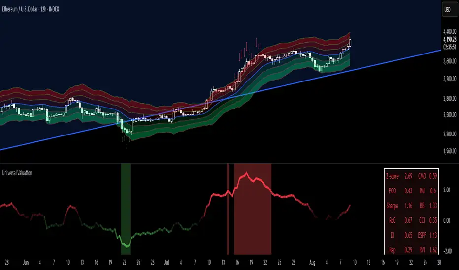
Universal Valuation[public code]Universal valuation indicator for all assets. Consists of 12 different indicators which are z-scored and averaged out.
> Volatility bands via Keltner Channels with a NWMA
> Confluence when price > vol.bands and valuation is high/low. The confluence is marked with red arrows when above the upper third band(green when below the lower on the downside), and 50% transparency when between 2/3 band(green when below the lower 2/3 bands on the downside.)
> Can be used separately of course.
> Can be used as valuation of indicators, when possible. (eg. Global Liquidity index valuation)
Code is a mess a bit, but parts can be extracted and a new strategy/indicator can be made.
*Big probs to the creator of this indicator . Inspired by him. I want to make it possible for people to extrapolate and create their own indicators/strategies. And of course, so I can do the same.
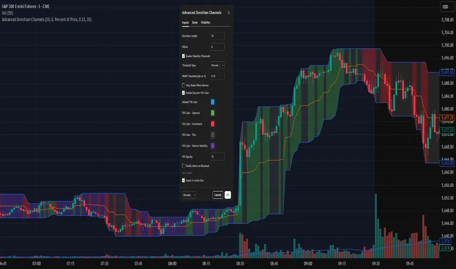
Advanced Donchian ChannelsJust an indicator I got ChatGPT to cook up for my own use, sharing it in case anyone else finds it useful. I have included a screenshot of my own settings as well for reference.
This indicator enhances the classic Donchian Channel with powerful contextual features to support modern breakout and volatility-based trading strategies.
🔹 Core Features:
Donchian Bands: Plots the highest high and lowest low over a configurable lookback period.
Dynamic Fill Shading:
- Color-coded based on the slope of the midline (Basis): Default settings are Green for uptrend, Red for downtrend, Silver for flat, Gray for narrow volatility.
- All fill colors are fully customizable.
Volatility Filter:
- Detects when the channel width is narrow using either a fixed value or a percentage of price.
- Optionally shades only during low-volatility (compression) periods.
Customizable Style:
- Adjustable opacity, offsets, and color settings to suit your charting style.
🛠 Use Cases:
- Spot potential breakout setups after periods of low volatility.
- Identify trend direction via basis slope shading.
- Combine with momentum or volume tools for high-probability entries.
Flashtrader´s Statistical BandwidthsThe vast majority of traders exclusively concern
themselves with trend-following in all its facets. Scoring
points with trends on a regular basis is a difficult task
since prices do not constantly move in one direction
or another. In the case of the DAX future, for example,
only about 30 per cent of all trading days in a year are
trend days. And of these, there are x percent long ones
and x per cent short ones. Catching the very days when
prices rise or fall from the opening to the close is a major
challenge for a trader who also needs to have previously
recognised the corresponding direction.
However, there are also other ways of profit-taking
every day – for example, by using the mean reversion
strategy. The idea behind this is the fact that prices reach
a high and a low every day – but very rarely close at the
high or the low. This means that prices always move
away from these extreme points and the closing price is
somewhere in between. A profitable trading strategy can
be developed out of this.
But how can you know where the high and the low
will be tomorrow? Is it possible for you to know this in
advance? No – because no one can predict the future. Or
can they? At least it can be statistically determined how
high or low prices could go tomorrow. There is a high
degree of probability that one of the two possibilities
will materialise. It will then be necessary to act.
Calculation
Classic pivot points for the following day are calculated
from the high, low and closing price. But does it really
make sense to use such a mix? I don’t think so and
use a different calculation for this strategy. In a first step,
only the differences between the start and the high or low
are calculated on a daily basis. To avoid being dependent
on individual days and outliers, it is advisable to calculate,
in a second step, the average of these differences over
the past five days. Finally, this average will then be added
at the opening price of the current trading day for the
upper statistical bandwidth and subtracted for the lower
bandwidth.
upper bandwidth = oSTB (violet dashed line in the chart)
lower bandwidth = uSTB (violet dashedline in the chart)
The second interesting question is, if the previous day's high has been exceeded, how much further can the price rise from a mathematical/statistical point of view?
These calculated previous day highs expansions are shown as red dashed lines
Previous day's high expansion = VTHA
Previous day's low expansion = VTTA
For further orientation, the previous day's high (VTH) and the previous day's low (VTT) are shown in light blue dashed lines
And as a supplement, the previous day's close in the DAX Future at 10:00 p.m. VTSA in violet solid lines and the previous day's close in the cash register at 5:30 p.m. VTSN in yellow solid lines
Reaching the calculated extreme values does not mean that the trend has to change immediately, but there is at least temporary exhaustion potential with which you can earn a few points every day in the area of scalping.
Example for cheap entry long:
Example for cheap entry short:
Deutsch:
Die Masse der Trader beschäftigt sich ausschließlich mit Trendfolge in all ihren Facetten. Mit Trends regelmäßig zu punkten ist ein schwieriges Unterfangen, da die Kurse nicht ständig in die eine oder andere Richtung laufen. Beim DAX-Future zum Beispiel sind von allen Börsentagen im Jahr lediglich zirka 30 Prozent Trendtage. Davon sind dann auch noch x Prozent Long und x Prozent Short. Hier genau die Tage abzupassen, an denen die Kurse von Börsenbeginn bis zum Schluss steigen beziehungsweise fallen, ist eine große Herausforderung – wobei der Trader zuvor noch die entsprechende Richtung erkannt haben muss. Es gibt jedoch auch noch andere Methoden täglich Gewinne mitzunehmen, zum Beispiel mit der Mean-Reversion-Strategie (Mittelwertumkehr).
Hintergrund ist die Tatsache, dass die Kurse jeden Tag ein Hoch und ein Tief erreichen – aber sehr selten am Hoch oder am Tief schließen. Das bedeutet, dass die Preise sich immer wie der von diesen Extrempunkten wegbewegen und der Schlusskurs irgendwo dazwischen liegt. Hieraus lässt sich eine profitable Handelsstrategie entwickeln. Aber woher kannst Du wissen, wo morgen das Hoch und das Tief sein wird? Kannst Du das vorher schon wissen? Nein – denn niemand kann die Zukunft vorhersagen. Oder doch? Statistisch lässt sich zumindest bestimmen, wie hoch und wie tief die Kurse morgen steigen oder fallen könnten. Eine Seite wird mit sehr hoher Wahrscheinlichkeit ein treffen. Dann gilt es zu handeln.
Berechnung Klassischer Pivot-Punkte für den folgenden Tag werden aus Hoch, Tief und Schlusskurs berechnet. Aber ist es wirklich sinnvoll, einen solchen Mix zu verwenden? Ich finde das nicht und verwenden für diese Strategie eine andere Berechnung. Im ersten Schritt werden täglich die Differenzen nur vom Start bis zum Hoch beziehungsweise Tief errechnet. Um nicht von einzelnen Tagen und Ausreißern abhängig zu sein, empfiehlt es sich, in einem zweiten Schritt den Durchschnitt dieser Differenzen über die letzten fünf Tage zu errechnen. Zuletzt wird dann dieser Durchschnitt zum Eröffnungskurs des aktuellen Handelstages für die obere statistische Bandbreite addiert und für die untere Bandbreite subtrahiert.
Obere statistische Bandbreite = oSTB (violette gestrichelte Linie im Chart)
Untere statistische Bandbreite = uSTB (violette gestrichelte Linie im Chart)
Die zweite interessante Frage ist, wenn das Vortageshoch überschritten wurde, wie weit kann der Kurs dann noch steigen aus mathematisch/statistischer Sicht?
Diese berechneten Vortagesextremausdehnungen sind als rote gestrichelte Linien dargestellt
Vortageshochausdehnung = VTHA
Vortagestiefausdehnung = VTTA
Für die weitere Orientierung sind die Vortageshochs (VTH) und die Vortagestiefs (VTT) als hellblaue gestrichelte Linien abgebildet.
Als Ergänzung wird noch der Vortages Schluss im Dax Future um 22:00 Uhr VTSA mit einer violetten durchgezogenen Linie und der Kassamarktschluss um 17:30 Uhr mit einer gelben durchgezogenen Linie gezeigt.
Das Erreichen der berechneten Extremwerte bedeutet nicht, das der Trend sofort drehen muss, aber es sind zumindest temporäre Erschöpfungspotentiale mit denen sich im Bereich scalping täglich einige Punkte verdienen lassen.
Beispiel für günstigen Einstieg Long:
Beispiel für günstigen Einstieg Short:

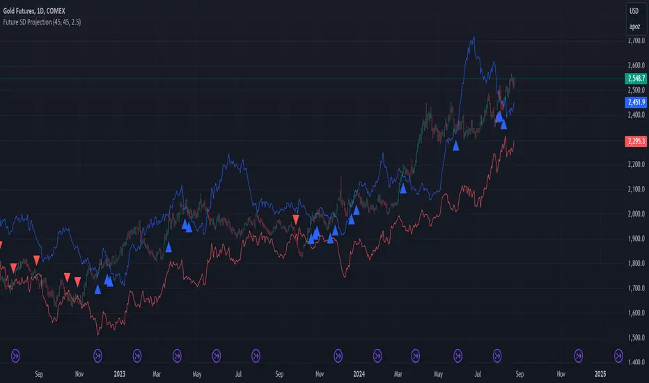
Future SD ProjectionFuture Standard Deviation Projector
This innovative indicator projects price volatility into the future, helping traders anticipate potential price ranges and breakouts. It calculates standard deviation bands based on recent price action and extends them forward, providing a unique perspective on future price movement possibilities.
Key Features:
- Projects standard deviation bands into the future
- Customizable lookback period for volatility calculation
- Adjustable future projection timeframe
- Flexible standard deviation multiplier
- Clear visual signals for band breaches
How it works:
1. Calculates standard deviation from recent closing prices
2. Projects upper and lower bands into the future
3. Plots these bands on the chart
4. Signals with arrows when closing price crosses projected bands
Use this indicator to:
- Gauge potential future price ranges
- Identify possible breakout levels
- Assess market volatility expectations
- Enhance your trading strategy with forward-looking volatility projections
Customize the settings to align with your trading timeframe and risk tolerance. Remember, while this tool offers valuable insights, it should be used in conjunction with other analysis methods for comprehensive trading decisions.
Note: Past performance and projections do not guarantee future results. Always manage your risk appropriately.
BabyShark VWAP Strategy What the code does:
This Pine Script implements a trading strategy based on two indicators: Volume Weighted Average Price (VWAP) and On Balance Volume (OBV) Relative Strength Index (RSI). The strategy aims to identify potential buy and sell signals based on deviations from VWAP and OBV RSI crossing certain threshold levels.
How it does it:
**VWAP Calculation**: The script calculates the VWAP using either standard deviation or average deviation over a specified length. It then plots the VWAP and its upper and lower deviation bands.
**OBV RSI Calculation**: It computes the OBV and then calculates the RSI using the cumulative changes in OBV. The RSI is plotted and compared against predefined levels.
**Table Visibility and Occurrence Counting**: It allows the user to display a table showing the number of occurrences where the price is above Upper Dev 2, below Lower Dev 2, crosses above a higher RSI level, or crosses below a lower RSI level.
**Entries**: Long and short entry conditions are defined based on the position of the price relative to the VWAP deviation bands and the color of the OBV RSI. Entries are made when specific conditions are met, and there hasn't been a recent entry.
**Exit Conditions**: The script includes stop-loss and take-profit mechanisms. It exits positions based on price crossing the VWAP or a certain percentage, and it prevents further trading after a certain number of consecutive losses.
What traders can use it for:
**Trend Identification**: Traders can use the VWAP and its deviation bands to identify potential trend reversals or continuations.
**Volume Confirmation**: The inclusion of OBV RSI provides confirmation of price movements based on volume changes.
**Entry and Exit Signals**: The script generates buy and sell signals based on the specified conditions, allowing traders to enter and exit positions with defined stop-loss and take-profit levels.
**Statistical Analysis**: The visibility of occurrence counts in the table allows traders to perform statistical analysis on the frequency of price movements relative to the VWAP and OBV RSI levels.

Multi VWAP for Wick HunterCredit: honeybadgermakesfunnymoney for this Open Source Script
Published:
This is a tool that will allow you to visualize Wick Hunter's calcation of VWAP. Wick Hunter uses this calcuation for its Liqudations Bots.
There are four settings that you need to be configured to visualize your VWAP Band:
Long VWAP - The distance from current VWAP price, in %, that price must be UNDER when a liquidation event occurs to meet your you VWAP condition. The higher the value, the more price must move below the current VWAP price for it to enter a LONG position.
Short VWAP - The distance from current VWAP price, in %, that price must be ABOVE when a liquidation event occurs to meet your you VWAP condition. The higher the value, the more price must move above the current VWAP price for it to enter a SHORT position.
VWAP Timeframe - Select the timeframe you want the VWAP to be measured on.
VWAP Periods: Input the time period over which you want the VWAP to be measured over. For example, if you use "5" for this and "15" for VWAP Timeframe. The VWAP will be calculated based on the last five 15 minute candles.
You can play around with these settings using the indicator provide above. The indicator will print a triangle when the conditon for VWAP is met for a long for short trade. Play around with these settings. A few good timeframes that are popular are 5 minute, 15 minute, and one hour (60 minute). As far as periods, the most common settings are between 5 periods and 15 periods. In general the lower the timeframe and periods and closer VWAP will follow price.

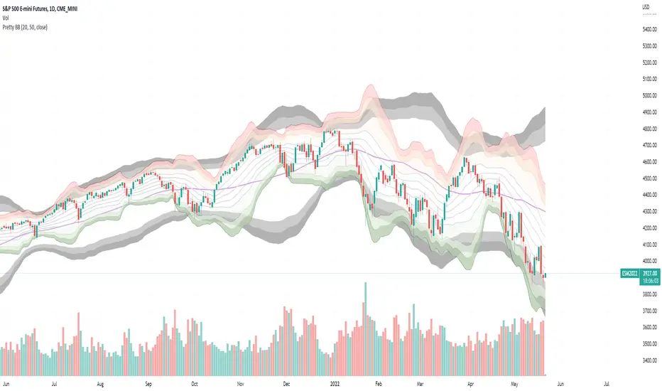
Pretty BollingersScheme shamelessly stolen from BORC. A pretty depiction of bollinger bands. Short basis plots from 5., 1, 2 (lines) deviations and then 2, 2.5, 3 (colored bands). Long basis plots only the basis, and 2, 2.5 and 3 bands (gray).
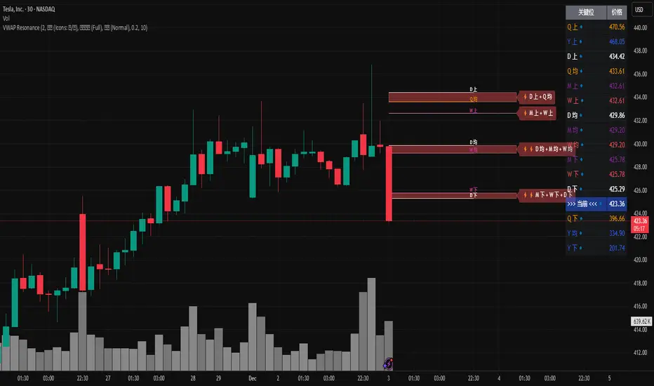
MTF VWAP Resonance [By Testeded]📈 MTF VWAP Resonance Hunter
(多级别 VWAP 共振捕猎者 - 终极版)
🇬🇧 English Description
1. Design Philosophy: The Institutional Edge
While typical indicators measure simple price action, VWAP (Volume Weighted Average Price) measures Value and Institutional Cost.
Professional traders and algorithms anchor their decisions to time-based benchmarks: Daily, Weekly, Monthly, and Quarterly. When prices return to these levels, they are testing the average cost basis of the market participants from that period.
The Logic of "Multi-Level Resonance" (MTF): A single VWAP line can be broken. However, when the Daily VWAP, Weekly Upper Band, and Quarterly Basis all overlap at the exact same price level, a "Market Consensus" is formed. This tool uses a background algorithm to detect these overlaps across 6 Timeframes (4H to Year) and visualizes them as "Resonance Boxes" instead of cluttering your chart with lines.
2. Key Features
⚓ Anchored VWAP Engine: Calculates VWAP + Standard Deviation Bands for 4H, Daily, Weekly, Monthly, Quarterly, and Yearly cycles simultaneously.
⚡ Smart Resonance Radar: Automatically detects when levels from different timeframes cluster together.
2-Line Confluence: ⚡ (Watch)
3-Line Confluence: ⚡⚡ (Strong)
4+ Line Confluence: ⚡⚡⚡ (Iron Wall)
🧘 Visual Modes (Zen / Focus):
Full Mode: Shows lines, dashboard, and resonance boxes.
Focus Mode: Hides lines, keeps dashboard and boxes.
Zen Mode: Hides EVERYTHING except the Resonance Boxes. Pure price action.
🏢 The Quarterly Line: Specifically designed to track the Quarterly VWAP, a critical level for institutional rebalancing and earnings cycles.
🎨 Customizable UI: Adjustable table text size (Small to Huge) and display styles.
3. How to Trade
Identify the Wall: Look for Red Boxes (Resistance) or Green Boxes (Support) with high star ratings (⚡⚡).
Read the Dashboard: Check the label (e.g., Q VWAP + W Lower). This tells you exactly who is defending this level (e.g., "Quarterly Buyers defending cost").
Sniper Entry: Wait for price to touch the Resonance Box. These levels often trigger sharp reversals or major breakouts.
🇨🇳 中文说明 (Chinese Description)
1. 设计哲学:多级别的全局视角
布林带反映的是波动率,而 VWAP(成交量加权平均价) 反映的是**“真金白银的持仓成本”**。
机构交易者和算法通常会锚定特定的时间周期进行交易:日内、周线、月线以及季度线。 “多级别共振”的逻辑: 单一周期的 VWAP 很容易失效。但是,当 日线 VWAP、周线上轨 和 季度线成本 在同一个价格位置重叠时,意味着短线、中线和长线资金在此处达成了**“价值共识”。 本指标通过后台算法,同时监控 6个时间周期 (4H - 年线),将这些重叠的价位转化为可视化的“共振框”**,提供一个多级别的全局视角。
2. 核心功能
⚓ 全周期锚定 VWAP:后台实时计算 4H, 日线, 周线, 月线, 季度线, 年线 的 VWAP 及其标准差轨道。
⚡ 智能共振雷达:自动检测不同周期的关键位重叠。
2线共振:⚡ (关注)
3线共振:⚡⚡ (强力支撑/阻力)
4线以上:⚡⚡⚡ (核弹级/铁壁共振)
🧘 显示模式 (Zen / Focus):
全面模式:显示所有线条 + 表格 + 共振框。
专注模式:隐藏线条,保留表格 + 共振框。
极简模式 (Zen):隐藏一切干扰,只显示共振框。像狙击手一样只看目标。
🏢 季度线增强:特别加入了 Quarterly VWAP (季度线),这是机构季末调仓和财报周期的重要防守线。
🎨 高度客制化:支持调整表格文字大小(从“小”到“巨大”),适配各种分辨率屏幕。
3. 实战用法
寻找“墙壁”:关注图表上的 红色共振框 (阻力) 或 绿色共振框 (支撑),尤其是带有 ⚡⚡ 标志的区域。
解读筹码:看一眼右上角的仪表盘标签(例如 Q VWAP + W Lower)。这意味着“季度级别的平均成本”与“周线级别的超卖线”重合,支撑力度极强。
警报交易:开启警报功能。不需要盯着屏幕,当价格撞上共振框时,指标会自动通知你。
BanditExperimental %R and Moving Average Bands. This is just for fun :)
Comment below if you spot a good pattern to trade.

ATR Overlay with Trailing Flip [ask2maniish]📘 ATR Overlay with Trailing Flip
🔍 Overview
The ATR Overlay with Trailing Flip is a dynamic, visually-enhanced overlay indicator designed to assist traders in trend detection, trailing stop management, and volatility-based decision making. It leverages the Average True Range (ATR) with optional dynamic multipliers, filters, and alerts to enhance trade execution precision.
⚙️ Features Summary
✅ Static & dynamic ATR multiplier
✅ Customizable trailing stop logic
✅ Volume & Bollinger Band filters
✅ Buy/Sell label signals with alerts
✅ ATR bands with color fill
✅ Optional candle coloring based on trend
✅ Table showing current ATR multiplier
✅ Fully customizable visual controls
🔧 User Inputs
📘 Info Panel
ATR Usage Guide
Tooltip with trading-style recommendations:
Scalping: ATR 5–10, Intraday: ATR 10–14 , Swing: ATR 14–21 , Position: ATR 21–50
📊 Visual Elements
📈 Plots
Upper/Lower ATR Bands
ATR Fill Zone
Dynamic Trailing Stop Line
🕯 Candle Coloring
Candles colored green (uptrend) or red (downtrend)
Wick coloring matches body
🏷 Signal Labels
"BUY" below candle when trend flips up
"SELL" above candle when trend flips down
📊 Table (Top Right)
Displays current multiplier value:
If static: Static: x.x
If dynamic: percentage format based on ATR ratio
🔔 Alerts
Two alert conditions:
Flip to Long → "📈 ATR flip to LONG"
Flip to Short → "📉 ATR flip to SHORT"
Sound can be enabled for real-time feedback.
🧠 Best Practices
Combine this tool with support/resistance or order flow indicators
Use dynamic ATR during volatile periods for better adaptability
Filter signals in ranging markets with BBand Width Filter
For scalping, reduce ATR period and multiplier for tighter risk
🛠️ Customization Tips
Adjust trailingPeriod for tighter/looser stops
Use color inputs to match your charting theme
Disable features (labels/fill) to declutter chart

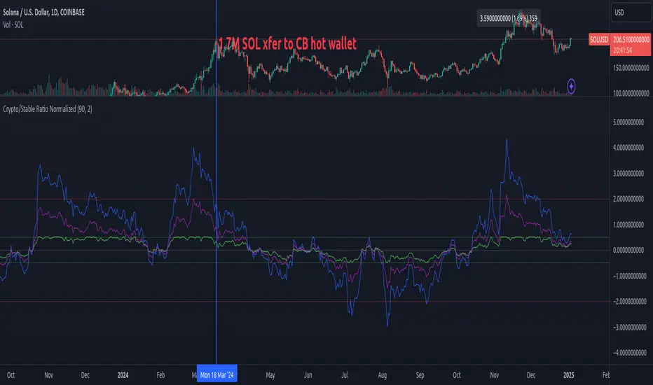
Crypto/Stable Mcap Ratio NormalizedCreate a normalized ratio of total crypto market cap to stablecoin supply (USDT + USDC + DAI). Idea is to create a reference point for the total market cap's position, relative to total "dollars" in the crypto ecosystem. It's an imperfect metric, but potentially helpful. V0.1.
This script provides four different normalization methods:
Z-Score Normalization:
Shows how many standard deviations the ratio is from its mean
Good for identifying extreme values
Mean-reverting properties
Min-Max Normalization:
Scales values between 0 and 1
Good for relative position within recent range
More sensitive to recent changes
Percent of All-Time Range:
Shows where current ratio is relative to all-time highs/lows
Good for historical context
Less sensitive to recent changes
Bollinger Band Position:
Similar to z-score but with adjustable sensitivity
Good for trading signals
Can be tuned via standard deviation multiplier
Features:
Adjustable lookback period
Reference bands for overbought/oversold levels
Built-in alerts for extreme values
Color-coded plots for easy visualization
PUBG//Pluto star appears on a chart when price goes in the in the extreme price range territory, i.e. beyond 2 standard deviation from the mean (or mid Bollinger Band).
//What makes a Pluto Star appear on a chart:
//1. Check if the candle 's' high and low, both are completely outside of the Bollinger Bands (close, 20, 2) - Lets call it Pluto Star Candle
//2. Pluto Star Candle must not be a result of sudden price movement. Hence the previous candle must give a BB Blast.
// In other words, the candle must have it's either open or close outside of Bollinger Bands, to confirm a BB Blast before the Pluto Star
//3. Candle, following the Pluto Star must not break the high (in case of upper BB i.e. short call) or low (in case of lower BB, i.e. long call), to confirm the reversal to the mean
// This implies that Pluto Star appears on chart, above/below the next candle of actual Pluto Star Candle

BTC Fair Value via Global Liquidity📈 BTC Fair Value via Global Liquidity
This indicator estimates Bitcoin's fair value based on a regression model using Global Liquidity (GLI) data from major central banks.
🔍 How it works:
Fair Value Line (orange): Calculated using a power-law model: Fair Value = e^b * (GLI)^a, where a and b are user-defined parameters based on historical regression.
Global Liquidity (GLI): Combines liquidity metrics from central banks (Fed, ECB, PBoC, BoJ, etc.), including adjustments for the RRP and TGA.
Deviation Bands (green/red dashed): Optional upper and lower bands showing % deviation from fair value (default ±25%). These help identify overbought/oversold conditions.
Delta Plot (gray dots): Displays the % deviation of BTC’s price from its modeled fair value.
⚙️ How to use:
Tune a and b for better model fitting (e.g., via log-log regression).
Use the deviation bands to identify potential entry/exit zones or periods of market inefficiency.
Ideal for macro-level BTC valuation and long-term strategic analysis.

Bollinger + EMA Strategy with StatsThis strategy is a mean-reversion trading model that combines Bollinger Band deviation entries with EMA-based exits. It enters a long position when the price drops significantly below the lower Bollinger Band by a user-defined multiple of standard deviation (x), and a short position when the price exceeds the upper band by the same logic. To manage risk, it uses a wider Bollinger Band threshold (y standard deviations) as a stop loss, while take profit occurs when the price reverts to the n-period EMA, indicating mean reversion. The strategy maintains only one active position at a time—either long or short—and allocates a fixed percentage of capital per trade. Performance metrics such as equity curve, drawdown, win rate, and total trades are tracked and displayed for backtesting evaluation.

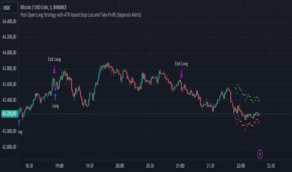
Post-Open Long Strategy with ATR-based Stop Loss and Take ProfitThe "Post-Open Long Strategy with ATR-Based Stop Loss and Take Profit" is designed to identify buying opportunities after the German and US markets open. It combines various technical indicators to filter entry signals, focusing on breakout moments following price lateralization periods.
Key Components and Their Interaction:
Bollinger Bands (BB):
Description: Uses BB with a 14-period length and standard deviation multiplier of 1.5, creating narrower bands for lower timeframes.
Role in the Strategy: Identifies low volatility phases (lateralization). The lateralization condition is met when the price is near the simple moving average of the BB, suggesting an imminent increase in volatility.
Exponential Moving Averages (EMA):
10-period EMA: Quickly detects short-term trend direction.
200-period EMA: Filters long-term trends, ensuring entries occur in a bullish market.
Interaction: Positions are entered only if the price is above both EMAs, indicating a consolidated positive trend.
Relative Strength Index (RSI):
Description: 7-period RSI with a threshold above 30.
Role in the Strategy: Confirms the market is not oversold, supporting the validity of the buy signal.
Average Directional Index (ADX):
Description: 7-period ADX with 7-period smoothing and a threshold above 10.
Role in the Strategy: Assesses trend strength. An ADX above 10 indicates sufficient momentum to justify entry.
Average True Range (ATR) for Dynamic Stop Loss and Take Profit:
Description: 14-period ATR with multipliers of 2.0 for Stop Loss and 4.0 for Take Profit.
Role in the Strategy: Adjusts exit levels based on current volatility, enhancing risk management.
Resistance Identification and Breakout:
Description: Analyzes the highs of the last 20 candles to identify resistance levels with at least two touches.
Role in the Strategy: A breakout above this level signals a potential continuation of the bullish trend.
Time Filters and Market Conditions:
Trading Hours: Operates only during the opening of the German market (8:00 - 12:00) and US market (15:30 - 19:00).
Panic Candle: The current candle must close negative, leveraging potential emotional reactions in the market.
Avoiding Entry During Pullbacks:
Description: Checks that the two previous candles are not both bearish.
Role in the Strategy: Avoids entering during a potential pullback, improving trade success probability.
Post-Open Long Strategy with ATR-Based Stop Loss and Take Profit
The "Post-Open Long Strategy with ATR-Based Stop Loss and Take Profit" is designed to identify buying opportunities after the German and US markets open. It combines various technical indicators to filter entry signals, focusing on breakout moments following price lateralization periods.
Key Components and Their Interaction:
Bollinger Bands (BB):
Description: Uses BB with a 14-period length and standard deviation multiplier of 1.5, creating narrower bands for lower timeframes.
Role in the Strategy: Identifies low volatility phases (lateralization). The lateralization condition is met when the price is near the simple moving average of the BB, suggesting an imminent increase in volatility.
Exponential Moving Averages (EMA):
10-period EMA: Quickly detects short-term trend direction.
200-period EMA: Filters long-term trends, ensuring entries occur in a bullish market.
Interaction: Positions are entered only if the price is above both EMAs, indicating a consolidated positive trend.
Relative Strength Index (RSI):
Description: 7-period RSI with a threshold above 30.
Role in the Strategy: Confirms the market is not oversold, supporting the validity of the buy signal.
Average Directional Index (ADX):
Description: 7-period ADX with 7-period smoothing and a threshold above 10.
Role in the Strategy: Assesses trend strength. An ADX above 10 indicates sufficient momentum to justify entry.
Average True Range (ATR) for Dynamic Stop Loss and Take Profit:
Description: 14-period ATR with multipliers of 2.0 for Stop Loss and 4.0 for Take Profit.
Role in the Strategy: Adjusts exit levels based on current volatility, enhancing risk management.
Resistance Identification and Breakout:
Description: Analyzes the highs of the last 20 candles to identify resistance levels with at least two touches.
Role in the Strategy: A breakout above this level signals a potential continuation of the bullish trend.
Time Filters and Market Conditions:
Trading Hours: Operates only during the opening of the German market (8:00 - 12:00) and US market (15:30 - 19:00).
Panic Candle: The current candle must close negative, leveraging potential emotional reactions in the market.
Avoiding Entry During Pullbacks:
Description: Checks that the two previous candles are not both bearish.
Role in the Strategy: Avoids entering during a potential pullback, improving trade success probability.
Entry and Exit Conditions:
Long Entry:
The price breaks above the identified resistance.
The market is in a lateralization phase with low volatility.
The price is above the 10 and 200-period EMAs.
RSI is above 30, and ADX is above 10.
No short-term downtrend is detected.
The last two candles are not both bearish.
The current candle is a "panic candle" (negative close).
Order Execution: The order is executed at the close of the candle that meets all conditions.
Exit from Position:
Dynamic Stop Loss: Set at 2 times the ATR below the entry price.
Dynamic Take Profit: Set at 4 times the ATR above the entry price.
The position is automatically closed upon reaching the Stop Loss or Take Profit.
How to Use the Strategy:
Application on Volatile Instruments:
Ideal for financial instruments that show significant volatility during the target market opening hours, such as indices or major forex pairs.
Recommended Timeframes:
Intraday timeframes, such as 5 or 15 minutes, to capture significant post-open moves.
Parameter Customization:
The default parameters are optimized but can be adjusted based on individual preferences and the instrument analyzed.
Backtesting and Optimization:
Backtesting is recommended to evaluate performance and make adjustments if necessary.
Risk Management:
Ensure position sizing respects risk management rules, avoiding risking more than 1-2% of capital per trade.
Originality and Benefits of the Strategy:
Unique Combination of Indicators: Integrates various technical metrics to filter signals, reducing false positives.
Volatility Adaptability: The use of ATR for Stop Loss and Take Profit allows the strategy to adapt to real-time market conditions.
Focus on Post-Lateralization Breakout: Aims to capitalize on significant moves following consolidation periods, often associated with strong directional trends.
Important Notes:
Commissions and Slippage: Include commissions and slippage in settings for more realistic simulations.
Capital Size: Use a realistic trading capital for the average user.
Number of Trades: Ensure backtesting covers a sufficient number of trades to validate the strategy (ideally more than 100 trades).
Warning: Past results do not guarantee future performance. The strategy should be used as part of a comprehensive trading approach.
With this strategy, traders can identify and exploit specific market opportunities supported by a robust set of technical indicators and filters, potentially enhancing their trading decisions during key times of the day.
Bollinger Stop StrategyClassic trading strategy using the Bollinger Bands indicator.
Strategy
Only stop orders are used to enter and exit the market.
If the price crossed the upper boundary of the Bollinger Bands, then enter into a long position (and close a short position).
If the price crosses the bottom of the Bollinger Bands, then enter short (and close a long position).
Short positions can be disabled (optional).
For
Crypto-currency market
Preferably coin/fiat (BTC/USD, ETH/USDT, etc)
Timeframe 1 day only
Settings
The original settings for the Bollinger Bands indicator are set by default.
Perhaps a better result will be if you use non-original price source.
Works well with OHLC4 and HLCC4.

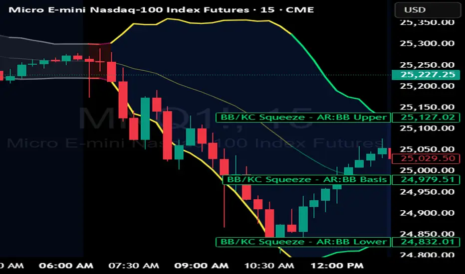
BB Keltner Squeeze - ArchReactorBollinger Band - Ketlner Squeeze .
Typical definition is when Bollinger band upper and lower is inside Ketlner channels , its when the squeeze happens.
Maybe helpful in developing strats around squeeze and the squeeze is displayed right on the chart.
Hurst Dual-Channel + ECDF Early Reentry (Single Trigger)Hello,
This indicator can be useful during ranging market phases, especially on short timeframes such as 5 minutes, within a statistically contrarian approach.
It combines two quantitative methodologies:
– Hurst-type adaptive channels, which measure short- and medium-term price deviations using the ATR (Average True Range);
– an Empirical Cumulative Distribution Function (ECDF), which locates the current price between its recent extremes (0 corresponding to the lower bound, 1 to the upper bound).
The goal is to identify relative overbought and oversold zones, where the price exceeds the channels and then begins to revert toward its statistical mean.
The indicator does not issue trading recommendations: it merely highlights specific statistical conditions for research and analytical purposes.
The “BUY” and “SELL” labels indicate such technical configurations:
– ECDF < 0.2 with price returning above the lower channels → bullish reentry.
– ECDF > 0.9 with price returning below the upper channels → bearish reentry.
The parameters (channel periods, ECDF window, smoothing) allow you to fine-tune the sensitivity of the analysis according to instrument volatility or chosen timeframe.
🟩 Buy Signal (BUY)
A buy signal is triggered when a strong downside deviation pushes the price below both channels, followed by a gradual reentry inside the bands.
More precisely:
– The low is below both channels (low < scb and low < mcb).
– The ECDF crosses back above 0.19 (exit from oversold).
– Both events occur within the last six bars.
– The price moves back above the lower channel (high > scb).
– No previous long signal is active.
This configuration represents a statistical reentry to the mean after an excessive drop.
🟥 Sell Signal (SELL)
Conversely, a sell signal appears when a strong upside deviation pushes the price above both channels, followed by a pullback below them:
– The high exceeds both channels (high > sct and high > mct).
– The ECDF crosses below 0.9 (exit from overbought).
– Both events occur within the last six bars.
– The price falls back below the upper channel (low < sct).
– No previous short signal is active.
This reflects a bearish reentry following a statistical overextension.
⚙️ Operating Logic
Each signal is triggered only once per cycle thanks to the variables triggered_long and triggered_short, preventing duplicates until a new extreme occurs.
The tool is designed for visual analysis and pattern research, not for automated execution.
🔍 ECDF Principle and Calculation
The ECDF is a non-parametric measure of a value’s position within its recent distribution:
ECDF(X)=number of values ≤XNECDF(X) = \frac{\text{number of values } \le X}{N}ECDF(X)=Nnumber of values ≤X
It expresses the empirical proportion of observations below the current value.
Example:
If, among the last 100 observations, 85 are below the current price, then
ECDF=0.85ECDF = 0.85ECDF=0.85
→ The price is at the 85th percentile, statistically high relative to recent history.
Strengths: robust, model-free, well-suited to asymmetric or non-normal market regimes.
Limitations: it does not measure amplitude and depends on the selected window size.
🌊 Intuitive Analogy: The River and the Gauge
Imagine a river with a depth gauge:
– The Z-Score tells you how many meters above the average level the water currently stands.
– The ECDF tells you in how many past cases the water level was lower than it is now.
The Z-Score assumes the river always follows the same symmetrical pattern.
The ECDF simply observes reality — adapting naturally, even when the current becomes unpredictable.
Final note:
This indicator is designed for visual and statistical exploration of price behavior.
The signals represent statistical states, not trade instructions.
Entering long or short positions based on them is entirely at your own discretion and risk.

Institutional Rolling VWAPs • 3 lines Institutional Rolling VWAPs • 3 lines + editable σ bands. 3 x modifiable vwaps, time anchored, same for ltf and htf

Plot_4_Key_LevelsBollinger Bands (upper & lower)
- computes 12-bar Bollinger Bands on the chart’s current timeframe, with a 3σ (standard-deviation) multiplier.
- computes vwap
- computes VWMA(HL2, 36)—a smoothed, volume-weighted average price—plotted as a line.
