VWAP Deviation Channels with Probability (Lite)VWAP Deviation Channels with Probability (Lite)
Version 1.2
Overview
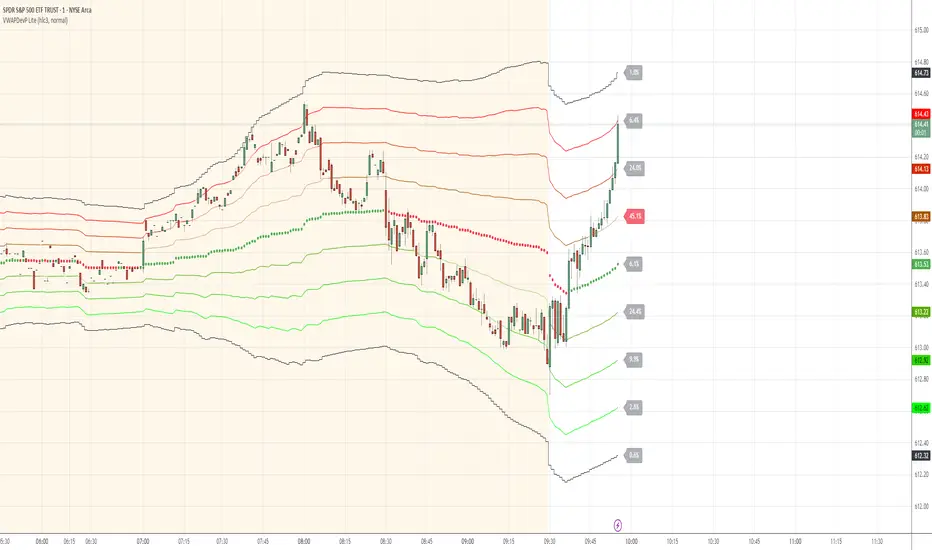
This indicator is a powerful tool for intraday traders, designed to identify high-probability areas of support and resistance. It plots the Volume-Weighted Average Price (VWAP) as a central "value" line and then draws statistically-based deviation channels around it.
Its unique feature is a dynamic probability engine that analyzes thousands of historical price bars to calculate and display the real-time likelihood of the price touching each of these deviation levels. This provides a quantifiable edge for making trading decisions.
Core Concepts Explained
This indicator is built on three key concepts:
The VWAP (Volume-Weighted Average Price): The dotted midline of the channels is the session VWAP. Unlike a Simple Moving Average (SMA) which only considers price, the VWAP incorporates volume into its calculation. This makes it a much more significant benchmark, as it represents the true average price where the most business has been transacted during the day. It's heavily used by institutional traders, which is why price often reacts strongly to it.
Standard Deviation Channels: The channels above and below the VWAP are based on standard deviations. Standard deviation is a statistical measure of volatility.
- Wide Bands: When the channels are wide, it signifies high volatility.
- Narrow Bands: When the channels are tight and narrow, it signifies low volatility and
consolidation (a "squeeze").
The Conditional Probability Engine: This is the heart of the indicator. For every deviation level, the script displays a percentage. This percentage answers a very specific question:
"Based on thousands of previous bars, when the last candle had a certain momentum (bullish or bearish), what was the historical probability that the price would touch this specific level?"
The probabilities are calculated separately depending on whether the previous candle was green (bullish) or red (bearish). This provides a nuanced, momentum-based edge. The level with the highest probability is highlighted, acting as a "price magnet."
How to Use This Indicator
Recommended Timeframes:
This indicator is designed specifically for intraday trading. It works best on timeframes like the 1-minute, 5-minute, and 15-minute charts. It will not display correctly on daily or higher timeframes.
Recommended Trading Strategy: Mean Reversion
The primary strategy for this indicator is "Mean Reversion." The core idea is that as the price stretches to extreme levels far away from the VWAP (the "mean"), it is statistically more likely to "snap back" toward it.
Here is a step-by-step guide to trading this setup:
1. Identify the Extreme: Wait for the price to push into one of the outer deviation bands (e.g., the -2, -3, or -4 bands for a buy setup, or the +2, +3, or +4 bands for a sell setup).
2. Look for the High-Probability Zone: Pay close attention to the highlighted probability label. This is the level that has historically acted as the strongest magnet for price. A touch of this level represents a high-probability area for a potential reversal.
3. Wait for Confirmation: Do not enter a trade just because the price has touched a band. Wait for a confirmation candle that shows momentum is shifting.
- For a Buy: Look for a strong bullish candle (e.g., a green engulfing candle or a hammer/pin
bar) to form at the lower bands.
- For a Sell: Look for a strong bearish candle (e.g., a red engulfing candle or a shooting star)
to form at the upper bands.
Define Your Exit:
- Take Profit: A logical primary target for a mean reversion trade is the VWAP (midLine).
- Stop Loss: A logical place for a stop-loss is just outside the next deviation band. For
example, if you enter a long trade at the -3 band, your stop loss could be placed just
below the -4 band.
Disclaimer: This indicator is a tool for analysis and should not be considered a standalone trading system. Trading involves significant risk, and past performance is not indicative of future results. Always use this indicator in conjunction with other forms of analysis and sound risk management practices.
ابحث في النصوص البرمجية عن "ha溢价率"
Rapid Candle PATTERNSIndicator Title: Rapid Candle Patterns - High-Probability Signals
Description
Tired of noisy charts filled with weak and ambiguous candlestick patterns? The Rapid Candle Patterns indicator is engineered to solve this problem by moving beyond simple textbook definitions. It identifies only high-probability reversal and continuation signals by focusing on the underlying market dynamics: momentum, liquidity, and confirmation.
This is not just another pattern indicator; it's a professional-grade tool designed to help you spot truly significant price action events.
How The Logic Works & Why It's More Accurate
Each pattern in this script has been enhanced with stricter, more intelligent rules to filter out noise and reduce false signals. Here’s what makes our logic superior:
1. The Liquidity Grab Hammer & Inverted Hammer
Standard Logic: A simple hammer shows a long lower wick, suggesting buyers pushed the price back up.
Our Enhanced Logic: We don't just look for a hammer shape. Our signal is only valid if the hammer’s low takes out the low of the previous candle (a "liquidity grab" or "stop hunt").
Why It's More Accurate: This sequence is incredibly powerful. It shows that sellers attempted to push the market lower, triggered stop-loss orders below the prior low, and then were decisively overpowered by buyers who reversed the price. This isn't just a reversal; it's a failed breakdown, often trapping sellers and fueling a stronger move in the opposite direction.
2. The "True" Bullish & Bearish Harami
Standard Logic: A small candle forms within the high-low range of the previous candle. This can often be misleading if the prior candle has long wicks and a tiny body.
Our Enhanced Logic: We enforce a "dual containment" rule. For a Harami to be valid, its body must be contained within the body of the previous candle. We also ensure the Harami candle itself is not a Doji, meaning it must show some conviction.
Why It's More Accurate: This ensures you are seeing a genuine and significant contraction in momentum. It filters out scenarios where a large-bodied candle forms inside the wicks of a doji-like candle, which is not a true Harami. Our logic captures the "pregnant" pattern as it was intended—a moment of quiet consolidation before a potential new move.
3. The "Power" Bullish & Bearish Engulfing
Standard Logic: A candle's body engulfs the body of the previous candle. This is a common signal, but it often lacks follow-through.
Our Enhanced Logic: Our "Power Engulfing" requires two conditions: (1) The body must engulf the prior candle's body, AND (2) the candle must close beyond the entire high/low range of the prior candle.
Why It's More Accurate: This is the ultimate sign of confirmation. It doesn't just show that one side has won the battle for the session; it proves they had enough force to break the entire structure of the previous candle. This signifies immense momentum and dramatically increases the probability that the trend will continue in the direction of the engulfing candle.
4. The Quantified Doji
Our Logic: Instead of being a subjective pattern, a Doji is defined quantitatively. It's a candle whose body is less than or equal to a user-defined percentage (default 9%) of its total range.
Why It's More Accurate: It provides a consistent and objective measure of market indecision. Furthermore, any candle identified as a Doji is automatically disqualified from being a Hammer, ensuring clear and distinct signals.
User Customization
Toggle Patterns On/Off: Declutter your chart by only showing the patterns you want to see.
Fine-Tune Logic: Use the "Pattern Logic" settings to adjust the sensitivity of the Doji and Harami detectors to perfectly match your trading style, asset, and timeframe.
Disclaimer: This indicator is a powerful tool for identifying high-probability price action. However, no single indicator is a complete trading system. Always use these signals as part of a comprehensive strategy, combined with analysis of market structure, support/resistance levels, and other forms of confluence.

CoffeeShopCrypto Supertrend Liquidity EngineMost SuperTrend indicators use fixed ATR multipliers that ignore context—forcing traders to constantly tweak settings that rarely adapt well across timeframes or assets.
This Supertrend is a nodd to and a more completion of the work
done by Olivier Seban ( @olivierseban )
This version replaces guesswork with an adaptive factor based on prior session volatility, dynamically adjusting stops to match current conditions. It also introduces liquidity-aware zones, real-time strength histograms, and a visual control panel—making your stoploss smarter, more responsive, and aligned with how the market actually moves.
📏 The Multiplier Problem & Adaptive Factor Solution
Traditional SuperTrend indicators rely on fixed ATR multipliers—often arbitrary numbers like 1.5, 2, or 3. The issue? No logical basis ties these values to actual market conditions. What works on a 5-minute Nasdaq chart fails on a daily EUR/USD chart. Traders spend hours tweaking multipliers per asset, timeframe, or volatility phase—and still end up with stoplosses that are either too tight or too loose. Worse, the market doesn’t care about your setting—it behaves according to underlying volatility, not your parameter.
This version fixes that by automating the multiplier selection entirely. It uses a 4-zone model based on the current ATR relative to the previous session’s ATR, dynamically adjusting the SuperTrend factor to match current volatility. It eliminates guesswork, adapts to the asset and timeframe, and ensures you’re always using a context-aware stoploss—one that evolves with the market instead of fighting it.
ATR EXAMPLE
Let’s say prior session ATR = 2.00
Now suppose current ATR = 0.32
This places us in Zone 1 (Very Low Volatility)
It doesn’t imply "overbought" or "oversold" — it tells you the market is moving very little, which often means:
Lower risk | Smaller stops | Smaller opportunities (and losses)
🔁 Liquidity Zones vs. Arbitrary Pullbacks
The standard SuperTrend stop loss line often looks like price “barely misses it” before continuing its trend. Traders call this "stop hunting," but what’s really happening is liquidity collection—price pulls back into a zone rich in orders before continuing. The problem? The old SuperTrend doesn’t show this zone. It only draws the outer limit, leaving no visual cue for where entries or continuation moves might realistically originate.
This script introduces 2 levels in the Liquidity Zone. One for Support and one for Stophunts, which draw dynamically between the current price and the SuperTrend line. These levels reflect where the market is most likely to revisit before resuming the trend. By visualizing the area just above the Supertrend stop loss, you can anticipate pullbacks, spot ideal re-entries, and avoid premature exits. This bridges the gap between mechanical stoploss logic and real-world liquidity behavior.
⏳ Prior Session ATR vs. Live ATR
Using real-time ATR to determine movement potential is like driving by looking in your rearview mirror. It’s reactive, not predictive. Traders often base decisions on live ATR, unaware that today’s range is still unfolding —creating volatility mismatches between what’s calculated and what actually matters. Since ATR reflects range, calculating it mid-session gives an incomplete and misleading picture of true volatility.
Instead, this system uses the ATR from the previous session , anchoring your volatility assumptions in a fully-formed price structure . It tells you how far price moved in the last full market phase—be it London, New York, or Tokyo—giving you a more reliable gauge of expected range today. This is a smarter way to estimate how far price could move rather than how far it has moved.
The Smoothing function will take the ATR, Support, Resistance, Stophunt Levels, and the Moving Avearage and smooth them by the calculation you choose.
It will also plot a moving average on your chart against closing prices by the smoothing function you choose.
🧭 Scalping vs. Trending Modes
The market moves in at least 4 phases. Trending, Ranging, Consolidation, Distribution.
Every trader has a different style —some scalp low-volatility moves during off-hours, while others ride macro trends across days. The problem with classic SuperTrend? It treats every market condition the same. A fixed system can’t possibly provide proper stoploss spacing for both a fast scalp and a long-term swing. Traders are forced to rebuild their system every time the market changes character or the session shifts.
This version solves that with a simple toggle:
Scalping or Trend Mode . With one switch, it inverts the logic of the adaptive factor to either tighten or loosen your trailing stops. During low-liquidity hours or consolidation phases, Scalping Mode offers snug stoplosses. During expansion or clear directional bias.
Trend Mode lets the trade breathe. This is flexibility built directly into the logic—not something you have to recalibrate manually.
📉 Histogram Oscillator for Move Strength
In legacy indicators, there’s no built-in way to gauge when the move is losing power . Traders rely on price action or momentum indicators to guess if a trend is fading. But this adds clutter, lag, and often contradiction. The classic SuperTrend doesn’t offer insight into how strong or weak the current trend leg is—only whether price has crossed a line.
This version includes a Trending Liquidity Histogram —a histogram that shows whether the liquidity in the SuperTrend zone is expanding or compressing. When the bars weaken or cross toward zero, it signals liquidity exhaustion . This early warning gives you time to prep for reversals or anticipate pullbacks. It even adapts visually depending on your trading mode, showing color-coded signals for scalping vs. trending behavior. It's both a strength gauge and a trade timing tool—built into your stoploss logic.
Histogram in Scalping Mode
Histogram in Trending Mode
📊 Visual Table for Real-Time Clarity
A major issue with custom indicators is opacity —you don’t always know what settings or values are currently being used. Even worse, if your dynamic logic changes mid-trade, you may not notice unless you go digging into the code or logs. This can create confusion, especially for discretionary traders.
This SuperTrend solves it with a clean visual summary table right on your chart. It shows your current ATR value, adaptive multiplier, trailing stop level, and whether a new zone size is active. That means no surprises and no second-guessing—everything important is visible and updated in real-time.
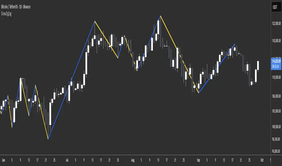
DrawZigZag🟩 OVERVIEW
This library draws zigzag lines for existing pivots. It is designed to be simple to use. If your script creates pivots and you want to join them up while handling edge cases, this library does that quickly and efficiently. If you want your pivots created for you, choose one of the many other zigzag libraries that do that.
🟩 HOW TO USE
Pine Script libraries contain reusable code for importing into indicators. You do not need to copy any code out of here. Just import the library and call the function you want.
For example, for version 1 of this library, import it like this:
import SimpleCryptoLife/DrawZigZag/1
See the EXAMPLE USAGE sections within the library for examples of calling the functions.
For more information on libraries and incorporating them into your scripts, see the Libraries section of the Pine Script User Manual.
🟩 WHAT IT DOES
I looked at every zigzag library on TradingView, after finishing this one. They all seemed to fall into two groups in terms of functionality:
• Create the pivots themselves, using a combination of Williams-style pivots and sometimes price distance.
• Require an array of pivot information, often in a format that uses user-defined types.
My library takes a completely different approach.
Firstly, it only does the drawing. It doesn't calculate the pivots for you. This isn't laziness. There are so many ways to define pivots and that should be up to you. If you've followed my work on market structure you know what I think of Williams pivots.
Secondly, when you pass information about your pivots to the library function, you only need the minimum of pivot information -- whether it's a High or Low pivot, the price, and the bar index. Pass these as normal variables -- bools, ints, and floats -- on the fly as your pivots confirm. It is completely agnostic as to how you derive your pivots. If they are confirmed an arbitrary number of bars after they happen, that's fine.
So why even bother using it if all it does it draw some lines?
Turns out there is quite some logic needed in order to connect highs and lows in the right way, and to handle edge cases. This is the kind of thing one can happily outsource.
🟩 THE RULES
• Zigs and zags must alternate between Highs and Lows. We never connect a High to a High or a Low to a Low.
• If a candle has both a High and Low pivot confirmed on it, the first line is drawn to the end of the candle that is the opposite to the previous pivot. Then the next line goes vertically through the candle to the other end, and then after that continues normally.
• If we draw a line up from a Low to a High pivot, and another High pivot comes in higher, we *extend* the line up, and the same for lines down. Yes this is a form of repainting. It is in my opinion the only way to end up with a correct structure.
• We ignore lower highs on the way up and higher lows on the way down.
🟩 WHAT'S COOL ABOUT THIS LIBRARY
• It's simple and lightweight: no exported user-defined types, no helper methods, no matrices.
• It's really fast. In my profiling it runs at about ~50ms, and changing the options (e.g., trimming the array) doesn't make very much difference.
• You only need to call one function, which does all the calculations and draws all lines.
• There are two variations of this function though -- one simple function that just draws lines, and one slightly more advanced method that modifies an array containing the lines. If you don't know which one you want, use the simpler one.
🟩 GEEK STUFF
• There are no dependencies on other libraries.
• I tried to make the logic as clear as I could and comment it appropriately.
• In the `f_drawZigZags` function, the line variable is declared using the `var` keyword *inside* the function, for simplicity. For this reason, it persists between function calls *only* if the function is called from the global scope or a local if block. In general, if a function is called from inside a loop , or multiple times from different contexts, persistent variables inside that function are re-initialised on each call. In this case, this re-initialisation would mean that the function loses track of the previous line, resulting in incorrect drawings. This is why you cannot call the `f_drawZigZags` function from a loop (not that there's any reason to). The `m_drawZigZagsArray` does not use any internal `var` variables.
• The function itself takes a Boolean parameter `_showZigZag`, which turns the drawings on and off, so there is no need to call the function conditionally. In the examples, we do call the functions from an if block, purely as an illustration of how to increase performance by restricting the amount of code that needs to be run.
🟩 BRING ON THE FUNCTIONS
f_drawZigZags(_showZigZag, _isHighPivot, _isLowPivot, _highPivotPrice, _lowPivotPrice, _pivotIndex, _zigzagWidth, _lineStyle, _upZigColour, _downZagColour)
This function creates or extends the latest zigzag line. Takes real-time information about pivots and draws lines. It does not calculate the pivots. It must be called once per script and cannot be called from a loop.
Parameters:
_showZigZag (bool) : Whether to show the zigzag lines.
_isHighPivot (bool) : Whether the current bar confirms a high pivot. Note that pivots are confirmed after the bar in which they occur.
_isLowPivot (bool) : Whether the current bar confirms a low pivot.
_highPivotPrice (float) : The price of the high pivot that was confirmed this bar. It is NOT the high price of the current bar.
_lowPivotPrice (float) : The price of the low pivot that was confirmed this bar. It is NOT the low price of the current bar.
_pivotIndex (int) : The bar index of the pivot that was confirmed this bar. This is not an offset. It's the `bar_index` value of the pivot.
_zigzagWidth (int) : The width of the zigzag lines.
_lineStyle (string) : The style of the zigzag lines.
_upZigColour (color) : The colour of the up zigzag lines.
_downZagColour (color) : The colour of the down zigzag lines.
Returns: The function has no explicit returns. As a side effect, it draws or updates zigzag lines.
method m_drawZigZagsArray(_a_zigZagLines, _showZigZag, _isHighPivot, _isLowPivot, _highPivotPrice, _lowPivotPrice, _pivotIndex, _zigzagWidth, _lineStyle, _upZigColour, _downZagColour, _trimArray)
Namespace types: array
Parameters:
_a_zigZagLines (array)
_showZigZag (bool) : Whether to show the zigzag lines.
_isHighPivot (bool) : Whether the current bar confirms a high pivot. Note that pivots are usually confirmed after the bar in which they occur.
_isLowPivot (bool) : Whether the current bar confirms a low pivot.
_highPivotPrice (float) : The price of the high pivot that was confirmed this bar. It is NOT the high price of the current bar.
_lowPivotPrice (float) : The price of the low pivot that was confirmed this bar. It is NOT the low price of the current bar.
_pivotIndex (int) : The bar index of the pivot that was confirmed this bar. This is not an offset. It's the `bar_index` value of the pivot.
_zigzagWidth (int) : The width of the zigzag lines.
_lineStyle (string) : The style of the zigzag lines.
_upZigColour (color) : The colour of the up zigzag lines.
_downZagColour (color) : The colour of the down zigzag lines.
_trimArray (bool) : If true, the array of lines is kept to a maximum size of two lines (the line elements are not deleted). If false (the default), the array is kept to a maximum of 500 lines (the maximum number of line objects a single Pine script can display).
Returns: This function has no explicit returns but it modifies a global array of zigzag lines.
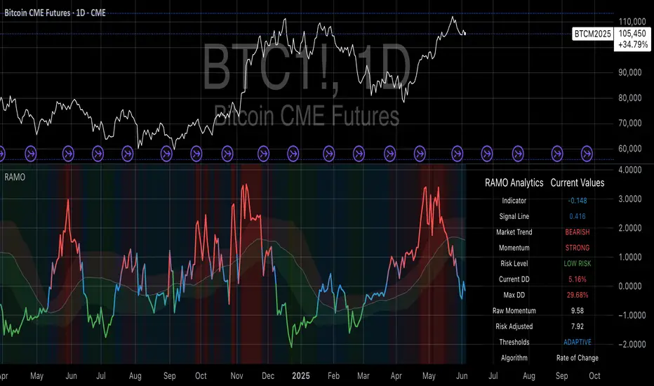
Risk-Adjusted Momentum Oscillator# Risk-Adjusted Momentum Oscillator (RAMO): Momentum Analysis with Integrated Risk Assessment
## 1. Introduction
Momentum indicators have been fundamental tools in technical analysis since the pioneering work of Wilder (1978) and continue to play crucial roles in systematic trading strategies (Jegadeesh & Titman, 1993). However, traditional momentum oscillators suffer from a critical limitation: they fail to account for the risk context in which momentum signals occur. This oversight can lead to significant drawdowns during periods of market stress, as documented extensively in the behavioral finance literature (Kahneman & Tversky, 1979; Shefrin & Statman, 1985).
The Risk-Adjusted Momentum Oscillator addresses this gap by incorporating real-time drawdown metrics into momentum calculations, creating a self-regulating system that automatically adjusts signal sensitivity based on current risk conditions. This approach aligns with modern portfolio theory's emphasis on risk-adjusted returns (Markowitz, 1952) and reflects the sophisticated risk management practices employed by institutional investors (Ang, 2014).
## 2. Theoretical Foundation
### 2.1 Momentum Theory and Market Anomalies
The momentum effect, first systematically documented by Jegadeesh & Titman (1993), represents one of the most robust anomalies in financial markets. Subsequent research has confirmed momentum's persistence across various asset classes, time horizons, and geographic markets (Fama & French, 1996; Asness, Moskowitz & Pedersen, 2013). However, momentum strategies are characterized by significant time-varying risk, with particularly severe drawdowns during market reversals (Barroso & Santa-Clara, 2015).
### 2.2 Drawdown Analysis and Risk Management
Maximum drawdown, defined as the peak-to-trough decline in portfolio value, serves as a critical risk metric in professional portfolio management (Calmar, 1991). Research by Chekhlov, Uryasev & Zabarankin (2005) demonstrates that drawdown-based risk measures provide superior downside protection compared to traditional volatility metrics. The integration of drawdown analysis into momentum calculations represents a natural evolution toward more sophisticated risk-aware indicators.
### 2.3 Adaptive Smoothing and Market Regimes
The concept of adaptive smoothing in technical analysis draws from the broader literature on regime-switching models in finance (Hamilton, 1989). Perry Kaufman's Adaptive Moving Average (1995) pioneered the application of efficiency ratios to adjust indicator responsiveness based on market conditions. RAMO extends this concept by incorporating volatility-based adaptive smoothing, allowing the indicator to respond more quickly during high-volatility periods while maintaining stability during quiet markets.
## 3. Methodology
### 3.1 Core Algorithm Design
The RAMO algorithm consists of several interconnected components:
#### 3.1.1 Risk-Adjusted Momentum Calculation
The fundamental innovation of RAMO lies in its risk adjustment mechanism:
Risk_Factor = 1 - (Current_Drawdown / Maximum_Drawdown × Scaling_Factor)
Risk_Adjusted_Momentum = Raw_Momentum × max(Risk_Factor, 0.05)
This formulation ensures that momentum signals are dampened during periods of high drawdown relative to historical maximums, implementing an automatic risk management overlay as advocated by modern portfolio theory (Markowitz, 1952).
#### 3.1.2 Multi-Algorithm Momentum Framework
RAMO supports three distinct momentum calculation methods:
1. Rate of Change: Traditional percentage-based momentum (Pring, 2002)
2. Price Momentum: Absolute price differences
3. Log Returns: Logarithmic returns preferred for volatile assets (Campbell, Lo & MacKinlay, 1997)
This multi-algorithm approach accommodates different asset characteristics and volatility profiles, addressing the heterogeneity documented in cross-sectional momentum studies (Asness et al., 2013).
### 3.2 Leading Indicator Components
#### 3.2.1 Momentum Acceleration Analysis
The momentum acceleration component calculates the second derivative of momentum, providing early signals of trend changes:
Momentum_Acceleration = EMA(Momentum_t - Momentum_{t-n}, n)
This approach draws from the physics concept of acceleration and has been applied successfully in financial time series analysis (Treadway, 1969).
#### 3.2.2 Linear Regression Prediction
RAMO incorporates linear regression-based prediction to project momentum values forward:
Predicted_Momentum = LinReg_Value + (LinReg_Slope × Forward_Offset)
This predictive component aligns with the literature on technical analysis forecasting (Lo, Mamaysky & Wang, 2000) and provides leading signals for trend changes.
#### 3.2.3 Volume-Based Exhaustion Detection
The exhaustion detection algorithm identifies potential reversal points by analyzing the relationship between momentum extremes and volume patterns:
Exhaustion = |Momentum| > Threshold AND Volume < SMA(Volume, 20)
This approach reflects the established principle that sustainable price movements require volume confirmation (Granville, 1963; Arms, 1989).
### 3.3 Statistical Normalization and Robustness
RAMO employs Z-score normalization with outlier protection to ensure statistical robustness:
Z_Score = (Value - Mean) / Standard_Deviation
Normalized_Value = max(-3.5, min(3.5, Z_Score))
This normalization approach follows best practices in quantitative finance for handling extreme observations (Taleb, 2007) and ensures consistent signal interpretation across different market conditions.
### 3.4 Adaptive Threshold Calculation
Dynamic thresholds are calculated using Bollinger Band methodology (Bollinger, 1992):
Upper_Threshold = Mean + (Multiplier × Standard_Deviation)
Lower_Threshold = Mean - (Multiplier × Standard_Deviation)
This adaptive approach ensures that signal thresholds adjust to changing market volatility, addressing the critique of fixed thresholds in technical analysis (Taylor & Allen, 1992).
## 4. Implementation Details
### 4.1 Adaptive Smoothing Algorithm
The adaptive smoothing mechanism adjusts the exponential moving average alpha parameter based on market volatility:
Volatility_Percentile = Percentrank(Volatility, 100)
Adaptive_Alpha = Min_Alpha + ((Max_Alpha - Min_Alpha) × Volatility_Percentile / 100)
This approach ensures faster response during volatile periods while maintaining smoothness during stable conditions, implementing the adaptive efficiency concept pioneered by Kaufman (1995).
### 4.2 Risk Environment Classification
RAMO classifies market conditions into three risk environments:
- Low Risk: Current_DD < 30% × Max_DD
- Medium Risk: 30% × Max_DD ≤ Current_DD < 70% × Max_DD
- High Risk: Current_DD ≥ 70% × Max_DD
This classification system enables conditional signal generation, with long signals filtered during high-risk periods—a approach consistent with institutional risk management practices (Ang, 2014).
## 5. Signal Generation and Interpretation
### 5.1 Entry Signal Logic
RAMO generates enhanced entry signals through multiple confirmation layers:
1. Primary Signal: Crossover between indicator and signal line
2. Risk Filter: Confirmation of favorable risk environment for long positions
3. Leading Component: Early warning signals via acceleration analysis
4. Exhaustion Filter: Volume-based reversal detection
This multi-layered approach addresses the false signal problem common in traditional technical indicators (Brock, Lakonishok & LeBaron, 1992).
### 5.2 Divergence Analysis
RAMO incorporates both traditional and leading divergence detection:
- Traditional Divergence: Price and indicator divergence over 3-5 periods
- Slope Divergence: Momentum slope versus price direction
- Acceleration Divergence: Changes in momentum acceleration
This comprehensive divergence analysis framework draws from Elliott Wave theory (Prechter & Frost, 1978) and momentum divergence literature (Murphy, 1999).
## 6. Empirical Advantages and Applications
### 6.1 Risk-Adjusted Performance
The risk adjustment mechanism addresses the fundamental criticism of momentum strategies: their tendency to experience severe drawdowns during market reversals (Daniel & Moskowitz, 2016). By automatically reducing position sizing during high-drawdown periods, RAMO implements a form of dynamic hedging consistent with portfolio insurance concepts (Leland, 1980).
### 6.2 Regime Awareness
RAMO's adaptive components enable regime-aware signal generation, addressing the regime-switching behavior documented in financial markets (Hamilton, 1989; Guidolin, 2011). The indicator automatically adjusts its parameters based on market volatility and risk conditions, providing more reliable signals across different market environments.
### 6.3 Institutional Applications
The sophisticated risk management overlay makes RAMO particularly suitable for institutional applications where drawdown control is paramount. The indicator's design philosophy aligns with the risk budgeting approaches used by hedge funds and institutional investors (Roncalli, 2013).
## 7. Limitations and Future Research
### 7.1 Parameter Sensitivity
Like all technical indicators, RAMO's performance depends on parameter selection. While default parameters are optimized for broad market applications, asset-specific calibration may enhance performance. Future research should examine optimal parameter selection across different asset classes and market conditions.
### 7.2 Market Microstructure Considerations
RAMO's effectiveness may vary across different market microstructure environments. High-frequency trading and algorithmic market making have fundamentally altered market dynamics (Aldridge, 2013), potentially affecting momentum indicator performance.
### 7.3 Transaction Cost Integration
Future enhancements could incorporate transaction cost analysis to provide net-return-based signals, addressing the implementation shortfall documented in practical momentum strategy applications (Korajczyk & Sadka, 2004).
## References
Aldridge, I. (2013). *High-Frequency Trading: A Practical Guide to Algorithmic Strategies and Trading Systems*. 2nd ed. Hoboken, NJ: John Wiley & Sons.
Ang, A. (2014). *Asset Management: A Systematic Approach to Factor Investing*. New York: Oxford University Press.
Arms, R. W. (1989). *The Arms Index (TRIN): An Introduction to the Volume Analysis of Stock and Bond Markets*. Homewood, IL: Dow Jones-Irwin.
Asness, C. S., Moskowitz, T. J., & Pedersen, L. H. (2013). Value and momentum everywhere. *Journal of Finance*, 68(3), 929-985.
Barroso, P., & Santa-Clara, P. (2015). Momentum has its moments. *Journal of Financial Economics*, 116(1), 111-120.
Bollinger, J. (1992). *Bollinger on Bollinger Bands*. New York: McGraw-Hill.
Brock, W., Lakonishok, J., & LeBaron, B. (1992). Simple technical trading rules and the stochastic properties of stock returns. *Journal of Finance*, 47(5), 1731-1764.
Calmar, T. (1991). The Calmar ratio: A smoother tool. *Futures*, 20(1), 40.
Campbell, J. Y., Lo, A. W., & MacKinlay, A. C. (1997). *The Econometrics of Financial Markets*. Princeton, NJ: Princeton University Press.
Chekhlov, A., Uryasev, S., & Zabarankin, M. (2005). Drawdown measure in portfolio optimization. *International Journal of Theoretical and Applied Finance*, 8(1), 13-58.
Daniel, K., & Moskowitz, T. J. (2016). Momentum crashes. *Journal of Financial Economics*, 122(2), 221-247.
Fama, E. F., & French, K. R. (1996). Multifactor explanations of asset pricing anomalies. *Journal of Finance*, 51(1), 55-84.
Granville, J. E. (1963). *Granville's New Key to Stock Market Profits*. Englewood Cliffs, NJ: Prentice-Hall.
Guidolin, M. (2011). Markov switching models in empirical finance. In D. N. Drukker (Ed.), *Missing Data Methods: Time-Series Methods and Applications* (pp. 1-86). Bingley: Emerald Group Publishing.
Hamilton, J. D. (1989). A new approach to the economic analysis of nonstationary time series and the business cycle. *Econometrica*, 57(2), 357-384.
Jegadeesh, N., & Titman, S. (1993). Returns to buying winners and selling losers: Implications for stock market efficiency. *Journal of Finance*, 48(1), 65-91.
Kahneman, D., & Tversky, A. (1979). Prospect theory: An analysis of decision under risk. *Econometrica*, 47(2), 263-291.
Kaufman, P. J. (1995). *Smarter Trading: Improving Performance in Changing Markets*. New York: McGraw-Hill.
Korajczyk, R. A., & Sadka, R. (2004). Are momentum profits robust to trading costs? *Journal of Finance*, 59(3), 1039-1082.
Leland, H. E. (1980). Who should buy portfolio insurance? *Journal of Finance*, 35(2), 581-594.
Lo, A. W., Mamaysky, H., & Wang, J. (2000). Foundations of technical analysis: Computational algorithms, statistical inference, and empirical implementation. *Journal of Finance*, 55(4), 1705-1765.
Markowitz, H. (1952). Portfolio selection. *Journal of Finance*, 7(1), 77-91.
Murphy, J. J. (1999). *Technical Analysis of the Financial Markets: A Comprehensive Guide to Trading Methods and Applications*. New York: New York Institute of Finance.
Prechter, R. R., & Frost, A. J. (1978). *Elliott Wave Principle: Key to Market Behavior*. Gainesville, GA: New Classics Library.
Pring, M. J. (2002). *Technical Analysis Explained: The Successful Investor's Guide to Spotting Investment Trends and Turning Points*. 4th ed. New York: McGraw-Hill.
Roncalli, T. (2013). *Introduction to Risk Parity and Budgeting*. Boca Raton, FL: CRC Press.
Shefrin, H., & Statman, M. (1985). The disposition to sell winners too early and ride losers too long: Theory and evidence. *Journal of Finance*, 40(3), 777-790.
Taleb, N. N. (2007). *The Black Swan: The Impact of the Highly Improbable*. New York: Random House.
Taylor, M. P., & Allen, H. (1992). The use of technical analysis in the foreign exchange market. *Journal of International Money and Finance*, 11(3), 304-314.
Treadway, A. B. (1969). On rational entrepreneurial behavior and the demand for investment. *Review of Economic Studies*, 36(2), 227-239.
Wilder, J. W. (1978). *New Concepts in Technical Trading Systems*. Greensboro, NC: Trend Research.
Shooting Star ORB🧠 Indicator Name: "First Candle Shooting Star + ORB"
📌 Purpose
This indicator detects when the first candle of the day forms a Shooting Star pattern and then monitors for a breakout beyond its range. It visually marks the pattern and the breakout with boxes and provides real-time alerts and a status table.
🔍 What It Does Step-by-Step
1. 📅 Detects the Start of a New Trading Day
Uses ta.change(time("D")) to identify a new trading day.
When a new day starts, it checks if the very first candle of the session is a Shooting Star.
2. 🕯️ Identifies a Shooting Star Pattern
A candle is labeled a Shooting Star if:
It has a small body compared to the full candle range.
It has a long upper shadow at least 2× the body.
It has a short or tiny lower shadow.
All these criteria are adjustable through inputs.
3. 📦 Draws a Box for the First Candle Range
If a Shooting Star is found in the first candle of the day:
It draws a red shaded box covering the high and low of that candle.
The box visually marks the potential Opening Range.
4. 💥 Detects Breakout from Shooting Star Candle
After the first candle:
If price moves above or below the range by a specified % (like 1%), it flags a breakout.
A blue shaded box is drawn at the breakout candle for visual confirmation.
5. 🔔 Alerts
🔴 Shooting Star Detected: Alerts when the first candle is a shooting star.
🔵 Breakout Detected: Alerts when the price breaks out of the first candle’s range.
6. 📊 Displays Real-Time Info Table
A small table is shown on the chart:
🕯️ Pattern: “Shooting Star” or blank
💥 Breakout: “Yes” or “No”
⏱️ The timeframe being analyzed (e.g., “5” for 5-minute)

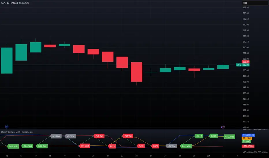
Chaikin Oscillator Multi-Timeframe BiasOverview
Chaikin Oscillator Multi-Timeframe Bias is an indicator designed to help traders align with institutional buying and selling activity by analyzing Chaikin Oscillator signals across two timeframes—a higher timeframe (HTF) for trend bias and a lower timeframe (LTF) for timing. This dual-confirmation model helps traders avoid false breakouts and trade in sync with market momentum and accumulation or distribution dynamics.
Core Concepts
The Chaikin Oscillator measures the momentum of accumulation and distribution based on price and volume. Institutional traders typically accumulate slowly and steadily, and the Chaikin Oscillator helps reveal this pattern. Multi-timeframe analysis confirms whether short-term price action supports the longer-term trend. This indicator applies a smoothing EMA to each Chaikin Oscillator to help confirm direction and reduce noise.
How to Use the Indicator
Start by selecting your timeframes. The higher timeframe, set by default to Daily, establishes the broader directional bias. The lower timeframe, defaulted to 30 minutes, identifies short-term momentum confirmation. The indicator displays one of five labels: CALL Bias, CALL Wait, PUT Bias, PUT Wait, or NEUTRAL. CALL Bias means both HTF and LTF are bullish, signaling a potential opportunity for long or call trades. CALL Wait indicates that the HTF is bullish, but the LTF hasn’t confirmed yet. PUT Bias signals bearish alignment in both HTF and LTF, while PUT Wait indicates HTF is bearish and LTF has not yet confirmed. NEUTRAL means there is no alignment between timeframes and directional trades are not advised.
Interpretation
When the Chaikin Oscillator is above zero and also above its EMA, this indicates bullish momentum and accumulation. When the oscillator is below zero and below its EMA, it suggests bearish momentum and distribution. Bias labels identify when both timeframes are aligned for a higher-probability directional setup. When a “Wait” label appears, it means one timeframe has confirmed bias but the other has not, suggesting the trader should monitor closely but delay entry.
Notes
This indicator includes alerts for both CALL and PUT bias confirmation when both timeframes are aligned. It works on all asset classes, including stocks, ETFs, cryptocurrencies, and futures. Timeframes are fully customizable, and users may explore combinations such as 1D and 1H, or 4H and 15M depending on their strategy. For best results, consider pairing this tool with volume, volatility, or price action analysis.
SMA50 ATR%SMA50 ATR% Zones Indicator
Overview:
The "SMA50 ATR%" indicator is designed to provide dynamic zones above and below a Simple Moving Average (SMA) based on multiples of the Average True Range (ATR). These zones can help traders identify potential areas of interest for entries, profit-taking, and stop-loss placement by visualizing how far the price has deviated from its medium-term mean (SMA) relative to its recent volatility (ATR).
Key Features:
Central SMA: Plots a customizable Simple Moving Average (default 50-period) as the baseline.
ATR-Based Zones: Calculates and displays distinct zones by adding or subtracting multiples of the ATR (default 10-period) from the SMA.
Color-Coded Visuals: Each zone type is clearly differentiated by color and shading intensity, providing an intuitive visual guide.
Current Zone Label: Displays the specific ATR multiple zone the current price is trading in, offering quick insight into the market's current position relative to the zones.
Zone Breakdown:
The indicator plots the following zones:
Entry Zones (Green Shades):
+1x ATR to +2x ATR above SMA
+2x ATR to +3x ATR above SMA
+3x ATR to +4x ATR above SMA
The green shades become progressively lighter as they move further from the SMA, with the zone closest to the SMA being the darkest green.
Hold Zones (Yellow Shades):
+4x ATR to +5x ATR above SMA (Darker Yellow)
+5x ATR to +6x ATR above SMA (Lighter Yellow)
Sell Zones (Red Shades):
+6x ATR to +7x ATR above SMA
+7x ATR to +8x ATR above SMA
+8x ATR to +9x ATR above SMA
+9x ATR to +10x ATR above SMA
+10x ATR to +11x ATR above SMA
The red shades become progressively darker as they move further from the +6x ATR level, with the +10x to +11x ATR zone being the darkest red.
Stop Loss Zones (Red Shades):
-1x ATR below SMA (Lighter Red)
-1x ATR to -2x ATR below SMA (Darker Red)
How to Use:
Potential Entry Areas: The green "Entry Zones" might indicate areas where the price has pulled back towards the SMA but is still showing strength, or areas where a breakout above the SMA is gaining momentum relative to volatility.
Potential Overbought/Hold Areas: The yellow "Hold Zones" could suggest that the price is becoming extended from its mean, warranting caution or a "hold" approach for existing positions.
Potential Profit-Taking/Sell Areas: The red "Sell Zones" might highlight significantly overbought conditions where the price has moved multiple ATRs above the SMA, potentially signaling areas for profit-taking or considering short entries.
Potential Stop-Loss Areas: The red "Stop Loss Zones" below the SMA can help define areas where a breakdown below the moving average, considering volatility, might invalidate a bullish bias.
Customization:
SMA Length: Adjust the period for the Simple Moving Average (Default: 50).
ATR Length: Adjust the period for the Average True Range calculation (Default: 10).
Show Current Zone Label: Toggle the visibility of the on-screen label that displays the current price's ATR zone.
SMA Line Width: Customize the thickness of the SMA line.
Label Position & Size: Control the placement and text size of the current zone label for optimal chart readability.
Disclaimer:
This indicator is a tool for technical analysis and should not be considered as financial advice. Always use risk management and combine with other analysis methods before making trading decisions.

magic wand STSM"Magic Wand STSM" Strategy: Trend-Following with Dynamic Risk Management
Overview:
The "Magic Wand STSM" (Supertrend & SMA Momentum) is an automated trading strategy designed to identify and capitalize on sustained trends in the market. It combines a multi-timeframe Supertrend for trend direction and potential reversal signals, along with a 200-period Simple Moving Average (SMA) for overall market bias. A key feature of this strategy is its dynamic position sizing based on a user-defined risk percentage per trade, and a built-in daily and monthly profit/loss tracking system to manage overall exposure and prevent overtrading.
How it Works (Underlying Concepts):
Multi-Timeframe Trend Confirmation (Supertrend):
The strategy uses two Supertrend indicators: one on the current chart timeframe and another on a higher timeframe (e.g., if your chart is 5-minute, the higher timeframe Supertrend might be 15-minute).
Trend Identification: The Supertrend's direction output is crucial. A negative direction indicates a bearish trend (price below Supertrend), while a positive direction indicates a bullish trend (price above Supertrend).
Confirmation: A core principle is that trades are only considered when the Supertrend on both the current and the higher timeframe align in the same direction. This helps to filter out noise and focus on stronger, more confirmed trends. For example, for a long trade, both Supertrends must be indicating a bearish trend (price below Supertrend line, implying an uptrend context where price is expected to stay above/rebound from Supertrend). Similarly, for short trades, both must be indicating a bullish trend (price above Supertrend line, implying a downtrend context where price is expected to stay below/retest Supertrend).
Trend "Readiness": The strategy specifically looks for situations where the Supertrend has been stable for a few bars (checking barssince the last direction change).
Long-Term Market Bias (200 SMA):
A 200-period Simple Moving Average is plotted on the chart.
Filter: For long trades, the price must be above the 200 SMA, confirming an overall bullish bias. For short trades, the price must be below the 200 SMA, confirming an overall bearish bias. This acts as a macro filter, ensuring trades are taken in alignment with the broader market direction.
"Lowest/Highest Value" Pullback Entries:
The strategy employs custom functions (LowestValueAndBar, HighestValueAndBar) to identify specific price action within the recent trend:
For Long Entries: It looks for a "buy ready" condition where the price has found a recent lowest point within a specific number of bars since the Supertrend turned bearish (indicating an uptrend). This suggests a potential pullback or consolidation before continuation. The entry trigger is a close above the open of this identified lowest bar, and also above the current bar's open.
For Short Entries: It looks for a "sell ready" condition where the price has found a recent highest point within a specific number of bars since the Supertrend turned bullish (indicating a downtrend). This suggests a potential rally or consolidation before continuation downwards. The entry trigger is a close below the open of this identified highest bar, and also below the current bar's open.
Candle Confirmation: The strategy also incorporates a check on the candle type at the "lowest/highest value" bar (e.g., closevalue_b < openvalue_b for buy signals, meaning a bearish candle at the low, suggesting a potential reversal before a buy).
Risk Management and Position Sizing:
Dynamic Lot Sizing: The lotsvalue function calculates the appropriate position size based on your Your Equity input, the Risk to Reward ratio, and your risk percentage for your balance % input. This ensures that the capital risked per trade remains consistent as a percentage of your equity, regardless of the instrument's volatility or price. The stop loss distance is directly used in this calculation.
Fixed Risk Reward: All trades are entered with a predefined Risk to Reward ratio (default 2.0). This means for every unit of risk (stop loss distance), the target profit is rr times that distance.
Daily and Monthly Performance Monitoring:
The strategy tracks todaysWins, todaysLosses, and res (daily net result) in real-time.
A "daily profit target" is implemented (day_profit): If the daily net result is very favorable (e.g., res >= 4 with todaysLosses >= 2 or todaysWins + todaysLosses >= 8), the strategy may temporarily halt trading for the remainder of the session to "lock in" profits and prevent overtrading during volatile periods.
A "monthly stop-out" (monthly_trade) is implemented: If the lres (overall net result from all closed trades) falls below a certain threshold (e.g., -12), the strategy will stop trading for a set period (one week in this case) to protect capital during prolonged drawdowns.
Trade Execution:
Entry Triggers: Trades are entered when all buy/sell conditions (Supertrend alignment, SMA filter, "buy/sell situation" candle confirmation, and risk management checks) are met, and there are no open positions.
Stop Loss and Take Profit:
Stop Loss: The stop loss is dynamically placed at the upTrendValue for long trades and downTrendValue for short trades. These values are derived from the Supertrend indicator, which naturally adjusts to market volatility.
Take Profit: The take profit is calculated based on the entry price, the stop loss, and the Risk to Reward ratio (rr).
Position Locks: lock_long and lock_short variables prevent immediate re-entry into the same direction once a trade is initiated, or after a trend reversal based on Supertrend changes.
Visual Elements:
The 200 SMA is plotted in yellow.
Entry, Stop Loss, and Take Profit lines are plotted in white, red, and green respectively when a trade is active, with shaded areas between them to visually represent risk and reward.
Diamond shapes are plotted at the bottom of the chart (green for potential buy signals, red for potential sell signals) to visually indicate when the buy_sit or sell_sit conditions are met, along with other key filters.
A comprehensive trade statistics table is displayed on the chart, showing daily wins/losses, daily profit, total deals, and overall profit/loss.
A background color indicates the active trading session.
Ideal Usage:
This strategy is best applied to instruments with clear trends and sufficient liquidity. Users should carefully adjust the Your Equity, Risk to Reward, and risk percentage inputs to align with their individual risk tolerance and capital. Experimentation with different ATR Length and Factor values for the Supertrend might be beneficial depending on the asset and timeframe.

Range Progress TrackerRANGE PROGRESS TRACKER(RPT)
PURPOSE
This indicator helps traders visually and statistically understand how much of the typical price range (measured by ATR) has already been covered in the current period (Daily, Weekly, or Monthly). It includes key features to assist in trend exhaustion analysis, reversal spotting, and smart alerting.
CORE LOGIC
The indicator calculates the current range of the selected time frame (e.g., Daily), which is:
Current Range = High - Low
This is then compared to the ATR (Average True Range) of the same time frame, which represents the average price movement range over a defined period (default is 14).
The comparison is expressed as a percentage, calculated with this formula:
Range % = (Current Range / ATR) × 100
This percentage shows how much of the “average expected move” has already occurred.
WHY IT MATTERS
When the current range approaches or exceeds 100% of ATR, it means the price has already moved as much as it typically does in a full session.
This indicates a lower probability of continuing the trend with a new high or low, especially when the price is already near the session's high or low.
This setup can signal:
A possible consolidation phase
A reversal in trend
The market entering a corrective phase
SMART ALERTS
The indicator can alert you when:
A new high is made after the range percentage exceeds your set threshold.
A new low is made after the range percentage exceeds your set threshold.
You can adjust the Range % Alert Threshold in the settings to tailor it to your trading style.

EMA Pullback Speed Strategy 📌 **Overview**
The **EMA Pullback Speed Strategy** is a trend-following approach that combines **price momentum** and **Exponential Moving Averages (EMA)**.
It aims to identify high-probability entry points during brief pullbacks within ongoing uptrends or downtrends.
The strategy evaluates **speed of price movement**, **relative position to dynamic EMA**, and **candlestick patterns** to determine ideal timing for entries.
One of the key concepts is checking whether the price has **“not pulled back too much”**, helping focus only on situations where the trend is likely to continue.
⚠️ This strategy is designed for educational and research purposes only. It does not guarantee future profits.
🧭 **Purpose**
This strategy addresses the common issue of **"jumping in too late during trends and taking unnecessary losses."**
By waiting for a healthy pullback and confirming signs of **trend resumption**, traders can enter with greater confidence and reduce false entries.
🎯 **Strategy Objectives**
* Enter in the direction of the prevailing trend to increase win rate
* Filter out false signals using pullback depth, speed, and candlestick confirmations
* Predefine Take-Profit (TP) and Stop-Loss (SL) levels for safer, rule-based trading
✨ **Key Features**
* **Dynamic EMA**: Reacts faster when price moves quickly, slower when market is calm – adapting to current momentum
* **Pullback Filter**: Avoids trades when price pulls back too far (e.g., more than 5%), indicating a trend may be weakening
* **Speed Check**: Measures how strongly the price returns to the trend using candlestick body speed (open-to-close range in ticks)
📊 **Trading Rules**
**■ Long Entry Conditions:**
* Current price is above the dynamic EMA (indicating uptrend)
* Price has pulled back toward the EMA (a "buy the dip" situation)
* Pullback depth is within the threshold (not excessive)
* Candlesticks show consecutive bullish closes and break the previous high
* Price speed is strong (positive movement with momentum)
**■ Short Entry Conditions:**
* Current price is below the dynamic EMA (indicating downtrend)
* Price has pulled back up toward the EMA (a "sell the rally" setup)
* Pullback is within range (not too deep)
* Candlesticks show consecutive bearish closes and break the previous low
* Price speed is negative (downward momentum confirmed)
**■ Exit Conditions (TP/SL):**
* **Take-Profit (TP):** Fixed 1.5% target above/below entry price
* **Stop-Loss (SL):** Based on recent price volatility, calculated using ATR × 4
💰 **Risk Management Parameters**
* Symbol & Timeframe: BTCUSD on 1-hour chart (H1)
* Test Capital: \$3000 (simulated account)
* Commission: 0.02%
* Slippage: 2 ticks (minimal execution lag)
* Max risk per trade: 5% of account balance
* Backtest Period: Aug 30, 2023 – May 9, 2025
* Profit Factor (PF): 1.965 (Net profit ÷ Net loss, including spreads & fees)
⚙️ **Trading Parameters & Indicator Settings**
* Maximum EMA Length: 50
* Accelerator Multiplier: 3.0
* Pullback Threshold: 5.0%
* ATR Period: 14
* ATR Multiplier (SL distance): 4.0
* Fixed TP: 1.5%
* Short-term EMA: 21
* Long-term EMA: 50
* Long Speed Threshold: ≥ 1000.0 (ticks)
* Short Speed Threshold: ≤ -1000.0 (ticks)
⚠️Adjustments are based on BTCUSD.
⚠️Forex and other currency pairs require separate adjustments.
🔧 **Strategy Improvements & Uniqueness**
Unlike basic moving average crossovers or RSI triggers, this strategy emphasizes **"momentum-supported pullbacks"**.
By combining dynamic EMA, speed checks, and candlestick signals, it captures trades **as if surfing the wave of a trend.**
Its built-in filters help **avoid overextended pullbacks**, which often signal the trend is ending – making it more robust than traditional trend-following systems.
✅ **Summary**
The **EMA Pullback Speed Strategy** is easy to understand, rule-based, and highly reproducible – ideal for both beginners and intermediate traders.
Because it shows **clear visual entry/exit points** on the chart, it’s also a great tool for practicing discretionary trading decisions.
⚠️ Past performance is not a guarantee of future results.
Always respect your Stop-Loss levels and manage your position size according to your risk tolerance.

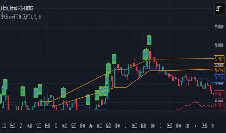
SMC Strategy BTC 1H - OB/FVGGeneral Context
This strategy is based on Smart Money Concepts (SMC), in particular:
The bullish Break of Structure (BOS), indicating a possible reversal or continuation of an upward trend.
The detection of Order Blocks (OB): consolidation zones preceding the BOS where the "smart money" has likely accumulated positions.
The detection of Fair Value Gaps (FVG), also called imbalance zones where the price has "jumped" a level, creating a disequilibrium between buyers and sellers.
Strategy Mechanics
Bullish Break of Structure (BOS)
A bullish BOS is detected when the price breaks a previous swing high.
A swing high is defined as a local peak higher than the previous 4 peaks.
Order Block (OB)
A bearish candle (close < open) just before a bullish BOS is identified as an OB.
This OB is recorded with its high and low.
An "active" OB zone is maintained for a certain number of bars (the zoneTimeout parameter).
Fair Value Gap (FVG)
A bullish FVG is detected if the high of the candle two bars ago is lower than the low of the current candle.
This FVG zone is also recorded and remains active for zoneTimeout bars.
Long Entry
An entry is possible if the price returns into the active OB zone or FVG zone (depending on which parameters are enabled).
Entry is only allowed if no position is currently open (strategy.position_size == 0).
Risk Management
The stop loss is placed below the OB low, with a buffer based on a multiple of the ATR (Average True Range), adjustable via the atrFactor parameter.
The take profit is set according to an adjustable Risk/Reward ratio (rrRatio) relative to the stop loss to entry distance.
Adjustable Parameters
Enable/disable entries based on OB and/or FVG.
ATR multiplier for stop loss.
Risk/Reward ratio for take profit.
Duration of OB and FVG zone activation.
Visualization
The script displays:
BOS (Break of Structure) with a green label above the candles.
OB zones (in orange) and FVG zones (in light blue).
Entry signals (green triangle below the candle).
Stop loss (red line) and take profit (green line).
Strengths and Limitations
Strengths:
Based on solid Smart Money analysis concepts.
OB and FVG zones are natural potential reversal areas.
Adjustable parameters allow optimization for different market conditions.
Dynamic risk management via ATR.
Limitations:
Only takes long positions.
No trend filter (e.g., EMA), which may lead to false signals in sideways markets.
Fixed zone duration may not fit all situations.
No automatic optimization; testing with different parameters is necessary.
Summary
This strategy aims to capitalize on price retracements into key zones where "smart money" has acted (OB and FVG) just after a bullish Break of Structure (BOS) signal. It is simple, customizable, and can serve as a foundation for a more comprehensive strategy.
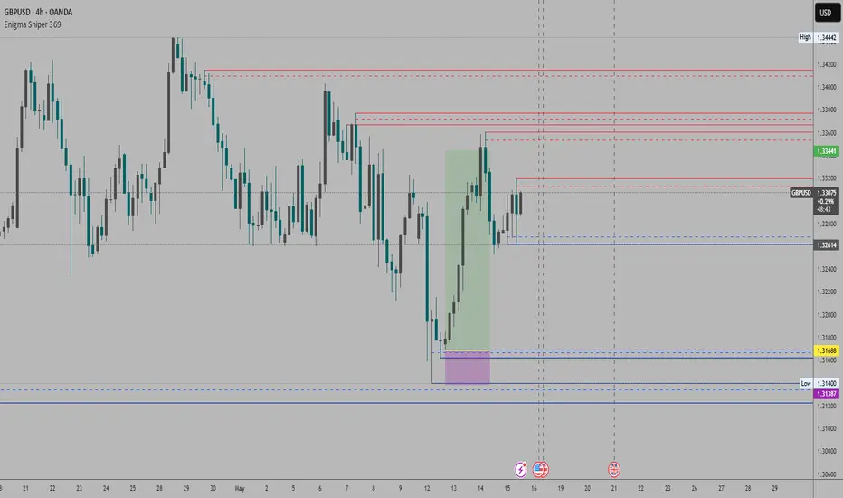
Enigma Sniper 369The "Enigma Sniper 369" is a custom-built Pine Script indicator designed for TradingView, tailored specifically for forex traders seeking high-probability entries during high-volatility market sessions.
Unlike generic trend-following or scalping tools, this indicator uniquely combines session-based "kill zones" (London and US sessions), momentum-based candle analysis, and an optional EMA trend filter to pinpoint liquidity grabs and reversal opportunities.
Its originality lies in its focus on liquidity hunting—identifying levels where stop losses are likely clustered (around swing highs/lows and wick midpoints)—and providing visual entry zones that are dynamically removed once price breaches them, reducing clutter and focusing on actionable signals.
The name "369" reflects the structured approach of three key components (session timing, candle logic, and trend filter) working in harmony to snipe precise entries.
What It Does
"Enigma Sniper 369" identifies potential buy and sell opportunities by drawing two types of horizontal lines on the chart during user-defined London and US
session kill zones:
Solid Lines: Mark the swing low (for buys) or swing high (for sells) of a trigger candle, indicating a potential entry point where stop losses might be clustered.
Dotted Lines: Mark the 50% level of the candle’s wick (lower wick for buys, upper wick for sells), serving as a secondary confirmation zone for entries or tighter stop-loss placement.
These lines are plotted only when specific candle conditions are met within the kill zones, and they are automatically deleted once the price crosses them, signaling that the liquidity at that level has likely been grabbed. The indicator also includes an optional EMA filter to ensure trades align with the broader trend, reducing false signals in choppy markets.
How It Works
The indicator’s logic is built on a multi-layered approach:
Kill Zone Timing: Trades are only considered during user-defined London and US session hours (e.g., London from 02:00 to 12:00 UTC, as seen in the screenshots). These sessions are known for high volatility and liquidity, making them ideal for capturing institutional moves.
Candle-Based Momentum Logic:
Buy Signal: A candle must close above its midpoint (indicating bullish momentum) and have a lower low than the previous candle (suggesting a potential liquidity grab below the previous swing low). This is expressed as close > (high + low) / 2 and low < low .
Sell Signal: A candle must close below its midpoint (bearish momentum) and have a higher high than the previous candle (indicating a potential liquidity grab above the previous swing high), expressed as close < (high + low) / 2 and high > high .
These conditions ensure the indicator targets candles that break recent structure to hunt stop losses while showing directional momentum.
Optional EMA Filter: A 50-period EMA (customizable) can be enabled to filter signals based on trend direction.
Buy signals are only generated if the EMA is trending upward (ema_value > ema_value ), and sell signals require a downward EMA trend (ema_value < ema_value ). This reduces noise by aligning entries with the broader market trend.
Liquidity Levels and Deletion Logic:
For a buy signal, a solid green line is drawn at the candle’s low, and a dotted green line at the 50% level of the lower wick (from the candle body’s bottom to the low).
For a sell signal, a solid red line is drawn at the candle’s high, and a dotted red line at the 50% level of the upper wick (from the body’s top to the high).
These lines extend to the right until the price crosses them, at which point they are deleted, indicating the liquidity at that level has been taken (e.g., stop losses triggered).
Alerts: The indicator includes alert conditions for buy and sell signals, notifying traders when a new setup is identified.
Underlying Concepts
The indicator is grounded in the concept of liquidity hunting, a strategy often employed by institutional traders. Markets frequently move to levels where stop losses are clustered—typically just beyond swing highs or lows—before reversing in the opposite direction. The "Enigma Sniper 369" targets these moves by identifying candles that break structure (e.g., a lower low or higher high) during high-volatility sessions, suggesting a potential sweep of stop losses. The 50% wick level acts as a secondary confirmation, as this midpoint often represents a zone where tighter stop losses are placed by retail traders. The optional EMA filter adds a trend-following element, ensuring entries are taken in the direction of the broader market momentum, which is particularly useful on lower timeframes like the 15-minute chart shown in the screenshots.
How to Use It
Here’s a step-by-step guide based on the provided usage example on the GBP/USD 15-minute chart:
Setup the Indicator: Add "Enigma Sniper 369" to your TradingView chart. Adjust the London and US session hours to match your timezone (e.g., London from 02:00 to 12:00 UTC, US from 13:00 to 22:00 UTC). Customize the EMA period (default 50) and line styles/colors if desired.
Identify Kill Zones: The indicator highlights the London session in light green and the US session in light purple, as seen in the screenshots. Focus on these periods for signals, as they are the most volatile and likely to produce liquidity grabs.
Wait for a Signal: Look for solid and dotted lines to appear during the kill zones:
Buy Setup: A solid green line at the swing low and a dotted green line at the 50% lower wick level indicate a potential buy. This suggests the market may have grabbed liquidity below the swing low and is now poised to move higher.
Sell Setup: A solid red line at the swing high and a dotted red line at the 50% upper wick level indicate a potential sell, suggesting liquidity was taken above the swing high.
Place Your Trade:
For a buy, set a buy limit order at the dotted green line (50% wick level), as this is a more conservative entry point. Place your stop loss just below the solid green line (swing low) to cover the full swing. For example, in the screenshots, the market retraces to the dotted line at 1.32980 after a liquidity grab below the swing low, triggering a buy limit order.
For a sell, set a sell limit order at the dotted red line, with a stop loss just above the solid red line.
Monitor Price Action: Once the price crosses a line, it is deleted, indicating the liquidity at that level has been taken. In the screenshots, after the buy limit is triggered, the market moves higher, confirming the setup. The caption notes, “The market returns and tags us in long with a buy limit,” highlighting this retracement strategy.
Additional Context: Use the indicator to identify liquidity levels that may be targeted later. For example, the screenshot notes, “If a new session is about to open I will wait for the grab liquidity to go long,” showing how the indicator can be used to anticipate future moves at session opens (e.g., London open at 1.32980).
Risk Management: Always set a stop loss below the swing low (for buys) or above the swing high (for sells) to protect against adverse moves. The 50% wick level helps tighten entries, improving the risk-reward ratio.
Practical Example
On the GBP/USD 15-minute chart, during the London session (02:00 UTC), the indicator identifies a buy setup with a solid green line at 1.32901 (swing low) and a dotted green line at 1.32980 (50% wick level). The market initially dips below the swing low, grabbing liquidity, then retraces to the dotted line, triggering a buy limit order. The price subsequently rises to 1.33404, yielding a profitable trade. The user notes, “The logic is in the last candle it provides new level to go long,” emphasizing the indicator’s ability to identify fresh levels after a liquidity sweep.
Customization Tips
Adjust the EMA period to suit your timeframe (e.g., a shorter period like 20 for faster signals on lower timeframes).
Modify the session hours to align with your broker’s timezone or specific market conditions.
Use the alert feature to get notified of new setups without constantly monitoring the chart.
Why It’s Useful for Traders
The "Enigma Sniper 369" stands out by combining session timing, momentum-based candle analysis, and liquidity hunting into a single tool. It provides clear, actionable levels for entries and stop losses, removes invalid signals dynamically, and aligns trades with high-probability market conditions. Whether you’re a scalper looking for quick moves during London open or a swing trader targeting session-based reversals, this indicator offers a structured, data-driven approach to trading.
IU Mean Reversion SystemDESCRIPTION
The IU Mean Reversion System is a dynamic mean reversion-based trading framework designed to identify optimal reversal zones using a smoothed mean and a volatility-adjusted band. This system captures price extremes by combining exponential and running moving averages with the Average True Range (ATR), effectively identifying overextended price action that is likely to revert back to its mean. It provides precise long and short entries with corresponding exit conditions, making it ideal for range-bound markets or phases of low volatility.
USER INPUTS :
Mean Length – Controls the smoothness of the mean; default is 9.
ATR Length – Defines the lookback period for ATR-based band calculation; default is 100.
Multiplier – Determines how wide the upper and lower bands are from the mean; default is 3.
LONG CONDITION :
A long entry is triggered when the closing price crosses above the lower band, indicating a potential upward mean reversion.
A position is taken only if there is no active long position already.
SHORT CONDITION :
A short entry is triggered when the closing price crosses below the upper band, signaling a potential downward mean reversion.
A position is taken only if there is no active short position already.
LONG EXIT :
A long position exits when the high price crosses above the mean, implying that price has reverted back to its average and may no longer offer favorable long risk-reward.
SHORT EXIT :
A short position exits when the low price crosses below the mean, indicating the mean reversion has occurred and the downside opportunity has likely played out.
WHY IT IS UNIQUE:
Uses a double smoothing approach (EMA + RMA) to define a stable mean, reducing noise and false signals.
Adapts dynamically to volatility using ATR-based bands, allowing it to handle different market conditions effectively.
Implements a state-aware entry system using persistent variables, avoiding redundant entries and improving clarity.
The logic is clear, concise, and modular, making it easy to modify or integrate with other systems.
HOW USER CAN BENEFIT FROM IT :
Traders can easily identify reversion opportunities in sideways or mean-reverting environments.
Entry and exit points are visually labeled on the chart, aiding in clarity and trade review.
Helps maintain discipline and consistency by using a rule-based framework instead of subjective judgment.
Can be combined with other trend filters, momentum indicators, or higher time frame context for enhanced results.

ADX Forecast [Titans_Invest]ADX Forecast
This isn’t just another ADX indicator — it’s the most powerful and complete ADX tool ever created, and without question the best ADX indicator on TradingView, possibly even the best in the world.
ADX Forecast represents a revolutionary leap in trend strength analysis, blending the timeless principles of the classic ADX with cutting-edge predictive modeling. For the first time on TradingView, you can anticipate future ADX movements using scientifically validated linear regression — a true game-changer for traders looking to stay ahead of trend shifts.
1. Real-Time ADX Forecasting
By applying least squares linear regression, ADX Forecast projects the future trajectory of the ADX with exceptional accuracy. This forecasting power enables traders to anticipate changes in trend strength before they fully unfold — a vital edge in fast-moving markets.
2. Unmatched Customization & Precision
With 26 long entry conditions and 26 short entry conditions, this indicator accounts for every possible ADX scenario. Every parameter is fully customizable, making it adaptable to any trading strategy — from scalping to swing trading to long-term investing.
3. Transparency & Advanced Visualization
Visualize internal ADX dynamics in real time with interactive tags, smart flags, and fully adjustable threshold levels. Every signal is transparent, logic-based, and engineered to fit seamlessly into professional-grade trading systems.
4. Scientific Foundation, Elite Execution
Grounded in statistical precision and machine learning principles, ADX Forecast upgrades the classic ADX from a reactive lagging tool into a forward-looking trend prediction engine. This isn’t just an indicator — it’s a scientific evolution in trend analysis.
⯁ SCIENTIFIC BASIS LINEAR REGRESSION
Linear Regression is a fundamental method of statistics and machine learning, used to model the relationship between a dependent variable y and one or more independent variables 𝑥.
The general formula for a simple linear regression is given by:
y = β₀ + β₁x + ε
β₁ = Σ((xᵢ - x̄)(yᵢ - ȳ)) / Σ((xᵢ - x̄)²)
β₀ = ȳ - β₁x̄
Where:
y = is the predicted variable (e.g. future value of RSI)
x = is the explanatory variable (e.g. time or bar index)
β0 = is the intercept (value of 𝑦 when 𝑥 = 0)
𝛽1 = is the slope of the line (rate of change)
ε = is the random error term
The goal is to estimate the coefficients 𝛽0 and 𝛽1 so as to minimize the sum of the squared errors — the so-called Random Error Method Least Squares.
⯁ LEAST SQUARES ESTIMATION
To minimize the error between predicted and observed values, we use the following formulas:
β₁ = /
β₀ = ȳ - β₁x̄
Where:
∑ = sum
x̄ = mean of x
ȳ = mean of y
x_i, y_i = individual values of the variables.
Where:
x_i and y_i are the means of the independent and dependent variables, respectively.
i ranges from 1 to n, the number of observations.
These equations guarantee the best linear unbiased estimator, according to the Gauss-Markov theorem, assuming homoscedasticity and linearity.
⯁ LINEAR REGRESSION IN MACHINE LEARNING
Linear regression is one of the cornerstones of supervised learning. Its simplicity and ability to generate accurate quantitative predictions make it essential in AI systems, predictive algorithms, time series analysis, and automated trading strategies.
By applying this model to the ADX, you are literally putting artificial intelligence at the heart of a classic indicator, bringing a new dimension to technical analysis.
⯁ VISUAL INTERPRETATION
Imagine an ADX time series like this:
Time →
ADX →
The regression line will smooth these values and extend them n periods into the future, creating a predicted trajectory based on the historical moment. This line becomes the predicted ADX, which can be crossed with the actual ADX to generate more intelligent signals.
⯁ SUMMARY OF SCIENTIFIC CONCEPTS USED
Linear Regression Models the relationship between variables using a straight line.
Least Squares Minimizes the sum of squared errors between prediction and reality.
Time Series Forecasting Estimates future values based on historical data.
Supervised Learning Trains models to predict outputs from known inputs.
Statistical Smoothing Reduces noise and reveals underlying trends.
⯁ WHY THIS INDICATOR IS REVOLUTIONARY
Scientifically-based: Based on statistical theory and mathematical inference.
Unprecedented: First public ADX with least squares predictive modeling.
Intelligent: Built with machine learning logic.
Practical: Generates forward-thinking signals.
Customizable: Flexible for any trading strategy.
⯁ CONCLUSION
By combining ADX with linear regression, this indicator allows a trader to predict market momentum, not just follow it.
ADX Forecast is not just an indicator — it is a scientific breakthrough in technical analysis technology.
⯁ Example of simple linear regression, which has one independent variable:
⯁ In linear regression, observations ( red ) are considered to be the result of random deviations ( green ) from an underlying relationship ( blue ) between a dependent variable ( y ) and an independent variable ( x ).
⯁ Visualizing heteroscedasticity in a scatterplot against 100 random fitted values using Matlab:
⯁ The data sets in the Anscombe's quartet are designed to have approximately the same linear regression line (as well as nearly identical means, standard deviations, and correlations) but are graphically very different. This illustrates the pitfalls of relying solely on a fitted model to understand the relationship between variables.
⯁ The result of fitting a set of data points with a quadratic function:
_______________________________________________________________________
🥇 This is the world’s first ADX indicator with: Linear Regression for Forecasting 🥇_______________________________________________________________________
_________________________________________________
🔮 Linear Regression: PineScript Technical Parameters 🔮
_________________________________________________
Forecast Types:
• Flat: Assumes prices will remain the same.
• Linreg: Makes a 'Linear Regression' forecast for n periods.
Technical Information:
ta.linreg (built-in function)
Linear regression curve. A line that best fits the specified prices over a user-defined time period. It is calculated using the least squares method. The result of this function is calculated using the formula: linreg = intercept + slope * (length - 1 - offset), where intercept and slope are the values calculated using the least squares method on the source series.
Syntax:
• Function: ta.linreg()
Parameters:
• source: Source price series.
• length: Number of bars (period).
• offset: Offset.
• return: Linear regression curve.
This function has been cleverly applied to the RSI, making it capable of projecting future values based on past statistical trends.
______________________________________________________
______________________________________________________
⯁ WHAT IS THE ADX❓
The Average Directional Index (ADX) is a technical analysis indicator developed by J. Welles Wilder. It measures the strength of a trend in a market, regardless of whether the trend is up or down.
The ADX is an integral part of the Directional Movement System, which also includes the Plus Directional Indicator (+DI) and the Minus Directional Indicator (-DI). By combining these components, the ADX provides a comprehensive view of market trend strength.
⯁ HOW TO USE THE ADX❓
The ADX is calculated based on the moving average of the price range expansion over a specified period (usually 14 periods). It is plotted on a scale from 0 to 100 and has three main zones:
• Strong Trend: When the ADX is above 25, indicating a strong trend.
• Weak Trend: When the ADX is below 20, indicating a weak or non-existent trend.
• Neutral Zone: Between 20 and 25, where the trend strength is unclear.
______________________________________________________
______________________________________________________
⯁ ENTRY CONDITIONS
The conditions below are fully flexible and allow for complete customization of the signal.
______________________________________________________
______________________________________________________
🔹 CONDITIONS TO BUY 📈
______________________________________________________
• Signal Validity: The signal will remain valid for X bars .
• Signal Sequence: Configurable as AND or OR .
🔹 +DI > -DI
🔹 +DI < -DI
🔹 +DI > ADX
🔹 +DI < ADX
🔹 -DI > ADX
🔹 -DI < ADX
🔹 ADX > Threshold
🔹 ADX < Threshold
🔹 +DI > Threshold
🔹 +DI < Threshold
🔹 -DI > Threshold
🔹 -DI < Threshold
🔹 +DI (Crossover) -DI
🔹 +DI (Crossunder) -DI
🔹 +DI (Crossover) ADX
🔹 +DI (Crossunder) ADX
🔹 +DI (Crossover) Threshold
🔹 +DI (Crossunder) Threshold
🔹 -DI (Crossover) ADX
🔹 -DI (Crossunder) ADX
🔹 -DI (Crossover) Threshold
🔹 -DI (Crossunder) Threshold
🔮 +DI (Crossover) -DI Forecast
🔮 +DI (Crossunder) -DI Forecast
🔮 ADX (Crossover) +DI Forecast
🔮 ADX (Crossunder) +DI Forecast
______________________________________________________
______________________________________________________
🔸 CONDITIONS TO SELL 📉
______________________________________________________
• Signal Validity: The signal will remain valid for X bars .
• Signal Sequence: Configurable as AND or OR .
🔸 +DI > -DI
🔸 +DI < -DI
🔸 +DI > ADX
🔸 +DI < ADX
🔸 -DI > ADX
🔸 -DI < ADX
🔸 ADX > Threshold
🔸 ADX < Threshold
🔸 +DI > Threshold
🔸 +DI < Threshold
🔸 -DI > Threshold
🔸 -DI < Threshold
🔸 +DI (Crossover) -DI
🔸 +DI (Crossunder) -DI
🔸 +DI (Crossover) ADX
🔸 +DI (Crossunder) ADX
🔸 +DI (Crossover) Threshold
🔸 +DI (Crossunder) Threshold
🔸 -DI (Crossover) ADX
🔸 -DI (Crossunder) ADX
🔸 -DI (Crossover) Threshold
🔸 -DI (Crossunder) Threshold
🔮 +DI (Crossover) -DI Forecast
🔮 +DI (Crossunder) -DI Forecast
🔮 ADX (Crossover) +DI Forecast
🔮 ADX (Crossunder) +DI Forecast
______________________________________________________
______________________________________________________
🤖 AUTOMATION 🤖
• You can automate the BUY and SELL signals of this indicator.
______________________________________________________
______________________________________________________
⯁ UNIQUE FEATURES
______________________________________________________
Linear Regression: (Forecast)
Signal Validity: The signal will remain valid for X bars
Signal Sequence: Configurable as AND/OR
Condition Table: BUY/SELL
Condition Labels: BUY/SELL
Plot Labels in the Graph Above: BUY/SELL
Automate and Monitor Signals/Alerts: BUY/SELL
Linear Regression (Forecast)
Signal Validity: The signal will remain valid for X bars
Signal Sequence: Configurable as AND/OR
Table of Conditions: BUY/SELL
Conditions Label: BUY/SELL
Plot Labels in the graph above: BUY/SELL
Automate & Monitor Signals/Alerts: BUY/SELL
______________________________________________________
📜 SCRIPT : ADX Forecast
🎴 Art by : @Titans_Invest & @DiFlip
👨💻 Dev by : @Titans_Invest & @DiFlip
🎑 Titans Invest — The Wizards Without Gloves 🧤
✨ Enjoy!
______________________________________________________
o Mission 🗺
• Inspire Traders to manifest Magic in the Market.
o Vision 𐓏
• To elevate collective Energy 𐓷𐓏
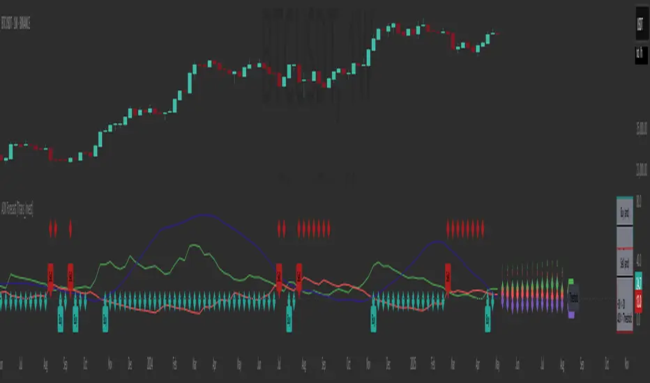
Zweig Market Breadth Thrust Indicator+Trigger [LazyBear x rwak]The Breadth Thrust (BT) indicator is a market momentum indicator developed by Dr. Martin Zweig. According to Dr. Zweig, a Breadth Thrust occurs when, during a 10-day period, the Breadth Thrust indicator rises from below 40 percent to above 61.5 percent.
A "Thrust" indicates that the stock market has rapidly changed from an oversold condition to one of strength, but has not yet become overbought. This is very rare and has happened only a few times. Dr. Zweig also points out that most bull markets begin with a Breadth Thrust.
This version of the Breadth Thrust indicator includes a trigger visualized with red circles, making it easier to spot when the indicator crosses the critical 61.5% level, signaling potential bullish momentum.
All parameters are configurable. You can draw BT for NYSE, NASDAQ, AMEX, or based on combined data (i.e., AMEX+NYSE+NASD). There is also a "CUSTOM" mode supported, so you can enter your own ADV/DEC symbols.
Credit: The original Breadth Thrust logic was created by LazyBear, whose public indicators can be found here , and app-store indicators here .
More info:
Definition of Breadth Thrust
A Breadth Thrust Signal
A Rare "Zweig" Buy Signal
Zweig Breadth Thrust: Redux
Frozen Bias Zones – Sentiment Lock-insOverview
The Frozen Bias Zones indicator visualizes market sentiment lock-ins using a combination of RSI, MACD, and OBV. It creates "bias zones" that indicate whether the market is in a sustained bullish or bearish phase. These zones are then highlighted on the chart, helping traders spot when the market is locked in a bias. The script also detects breakout events from these zones and marks them with clear labels for easier decision-making.
Features
Multi-Indicator Sentiment Analysis: Combines RSI, MACD, and OBV to detect synchronized bullish or bearish sentiment.
Frozen Bias Zones: Identifies and visually represents zones where the market has remained in a particular sentiment (bullish or bearish) for a defined period.
Breakout Alerts: Displays labels to indicate when the price breaks out of the established bias zone.
Customizable Inputs: Adjust the zone duration, RSI, MACD, and breakout label visibility.
Input Parameters
Bias Duration (biasLength)
The minimum number of candles the market must stay in a specific sentiment to consider it a "Frozen Bias Zone".
Default: 5 candles.
RSI Period (rsiPeriod)
Period for the Relative Strength Index (RSI) calculation.
Default: 14 periods.
MACD Settings
MACD Fast (macdFast): The fast-moving average period for the MACD calculation.
Default: 12.
MACD Slow (macdSlow): The slow-moving average period for the MACD calculation.
Default: 26.
MACD Signal (macdSig): The signal line period for MACD.
Default: 9.
Show Break Label (showBreakLabel)
Toggle to show labels when the price breaks out of the bias zone.
Default: True (shows label).
Bias Zone Colors
Bullish Bias Color (bullColor): The color for bullish zones (light green).
Bearish Bias Color (bearColor): The color for bearish zones (light red).
How It Works
This indicator analyzes three key market metrics to determine whether the market is in a bullish or bearish phase:
RSI (Relative Strength Index)
Measures the speed and change of price movements. RSI > 50 indicates a bullish phase, while RSI < 50 indicates a bearish phase.
MACD (Moving Average Convergence Divergence)
Measures the relationship between two moving averages of the price. A positive MACD histogram indicates bullish momentum, while a negative histogram indicates bearish momentum.
OBV (On-Balance Volume)
Uses volume flow to determine if a trend is likely to continue. A rising OBV indicates bullish accumulation, while a falling OBV indicates bearish distribution.
Bias Zone Detection
The market sentiment is considered bullish if all three indicators (RSI, MACD, and OBV) are bullish, and bearish if all three indicators are bearish.
Bullish Zone: A zone is created when the market sentiment remains bullish for the duration of the specified biasLength.
Bearish Zone: A zone is created when the market sentiment remains bearish for the duration of the specified biasLength.
These bias zones are visually represented on the chart as colored boxes (green for bullish, red for bearish).
Breakout Detection
The script automatically detects when the market exits a bias zone. If the price moves outside the bounds of the established zone (either up or down), the script will display one of the following labels:
Bias Break (Up): Indicates that the price has broken upwards out of the zone (with a green label).
Bias Break (Down): Indicates that the price has broken downwards out of the zone (with a red label).
These labels help traders easily identify potential breakout points.
Example Use Case
Bullish Market Conditions: If the RSI is above 50, the MACD histogram is positive, and OBV is increasing, the script will highlight a green bias zone. Traders can watch for potential bullish breakouts or trend continuation after the zone ends.
Bearish Market Conditions: If the RSI is below 50, the MACD histogram is negative, and OBV is decreasing, the script will highlight a red bias zone. Traders can look for potential bearish breakouts when the zone ends.
Conclusion
The Frozen Bias Zones indicator is a powerful tool for traders looking to visualize prolonged market sentiment, whether bullish or bearish. By combining RSI, MACD, and OBV, it helps traders spot when the market is "locked in" to a bias. The breakout labels make it easier to take action when the price moves outside of the established zone, potentially signaling the start of a new trend.
Instructions
To use this script:
Add the Frozen Bias Zones indicator to your TradingView chart.
Adjust the input parameters to suit your trading strategy.
Observe the colored bias zones on your chart, along with breakout labels, to make informed decisions on trend continuation or reversal.

Gap & Reversal Signals (Normal vs Heikin-Ashi)🔍 Gap & Reversal Signals (Normal vs Heikin-Ashi) — by
This script is designed to help traders identify key market signals by comparing Normal Candlestick Patterns with Heikin-Ashi values to highlight potential:
✅ Gap Up Opportunities (Strong Bullish Continuation)
🔻 Gap Down Alerts (Strong Bearish Continuation)
🔄 Bullish Reversal Zones (Possible Trend Reversal from Bearish to Bullish)
🔁 Bearish Reversal Zones (Possible Trend Reversal from Bullish to Bearish)
🧠 How it Works:
Gap Up: Normal candle is bullish, Heikin-Ashi is also bullish, and price closes higher than the HA close.
Gap Down: Normal candle is bearish, Heikin-Ashi is also bearish, and price closes lower than the HA close.
Bullish Reversal: Normal candle is bullish, but Heikin-Ashi shows bearish — potential reversal signal.
Bearish Reversal: Normal candle is bearish, but Heikin-Ashi shows bullish — potential reversal signal.
📊 Plot Details:
💚 Gap Up → Green Label Below Bar
❤️ Gap Down → Red Label Above Bar
💙 Bullish Reversal → Blue Label Below Bar
🧡 Bearish Reversal → Orange Label Above Bar
🚀 Use Cases:
Swing and positional traders looking for high-probability reversal setups
Intraday traders spotting early momentum shifts
Backtesters combining HA + candlestick logic for more robust strategies

RSI Support & Resistance Breakouts with OrderblocksThis tool is an overly simplified method of finding market squeeze and breakout completely based on a dynamic RSI calculation. It is designed to draw out areas of price levels where the market is pushing back against price action leaving behind instances of short term support and resistance levels you otherwise wouldn't see with the common RSI.
It uses the changes in market momentum to determine support and resistance levels in real time while offering price zone where order blocks exist in the short term.
In ranging markets we need to know a couple things.
1. External Zone - It's important to know where the highs and lows were left behind as they hold liquidity. Here you will have later price swings and more false breakouts.
2. Internal Zone - It's important to know where the highest and lowest closing values were so we can see the limitations of that squeeze. Here you will find the stronger cluster of orders often seen as orderblocks.
In this tool I've added a 200 period Smoothed Moving Average as a trend filter which causes the RSI calculation to change dynamically.
Regular Zones - without extending
The Zones draw out automatically but are often too small to work with.
To solve this problem, you can extend the zones into the future up to 40 bars.
This allows for more visibility against future price action.
--------------------------------------------
Two Types of Zones
External Zones - These zones give you positioning of the highest and lowest price traded within the ranging market. This is where liquidity will be swept and often is an ultimate breaking point for new price swings.
How to use them :
External Zones - External zones form at the top of a pullback. After this price should move back into its impulsive wave.
During the next corrective way, if price breaches the top of the previous External Zone, this is a sign of trend weakness. Expect a divergence and trend reversal.
Internal Zones - (OrderBlocks) Current price will move in relation to previous internal zones. The internal zone is where a majority of price action and trading took place. It's a stronger SQUEEZE area. Current price action will often have a hard time closing beyond the previous Internal Zones high or low. You can expect these zones to show you where the market will flip over. In these same internal zones you'll find large rejection candles.
**Important Note** Size Doesn't Matter
The size of the internal zone does not matter. It can be very small and still very powerful.
Once an internal zone has been hit a few times, its often not relevant any longer.
Order Block Zone Examples
In this image you can see the Internal Zone that was untouched had a STRONG price reaction later on.
Internal Zones that were touched multiple times had weak reactions later as price respected them less over time.
Zone Overlay Breakdown
The Zones form and update in real time until momentum has picked up and price begins to trend. However it leaves behind the elements of the inducement area and all the key levels you need to know about for future price action.
Resistance Fakeout : Later on after the zone has formed, price will return to this upper zone of price levels and cause fakeouts. A close above this zone implies the market moves long again.
Midline Equilibrium : This is simply the center of the strongest traded area. We can call this the Point of Control within the orderblock. If price expands through both extremes of this zone multiple times in the future, it eliminates the orderblock.
Support Fakeout : Just like its opposing brother, price will wick through this zone and rip back causing inducement to trap traders. You would need a clear close below this zone to be in a bearish trend.
BARCOLOR or Candle Color: (Optional)
Bars are colored under three conditions
Bullish Color = A confirmed bullish breakout of the range.
Bearish Color = A confirmed bearish breakout of the range.
Squeeze Color = Even if no box is formed a candle or candles can have a squeeze color. This means the ranging market happened within the high and low of that singular candle.
Z-Score Normalized VIX StrategyThis strategy leverages the concept of the Z-score applied to multiple VIX-based volatility indices, specifically designed to capture market reversals based on the normalization of volatility. The strategy takes advantage of VIX-related indicators to measure extreme levels of market fear or greed and adjusts its position accordingly.
1. Overview of the Z-Score Methodology
The Z-score is a statistical measure that describes the position of a value relative to the mean of a distribution in terms of standard deviations. In this strategy, the Z-score is calculated for various volatility indices to assess how far their values are from their historical averages, thus normalizing volatility levels. The Z-score is calculated as follows:
Z = \frac{X - \mu}{\sigma}
Where:
• X is the current value of the volatility index.
• \mu is the mean of the index over a specified period.
• \sigma is the standard deviation of the index over the same period.
This measure tells us how many standard deviations the current value of the index is away from its average, indicating whether the market is experiencing unusually high or low volatility (fear or calm).
2. VIX Indices Used in the Strategy
The strategy utilizes four commonly referenced volatility indices:
• VIX (CBOE Volatility Index): Measures the market’s expectations of 30-day volatility based on S&P 500 options.
• VIX3M (3-Month VIX): Reflects expectations of volatility over the next three months.
• VIX9D (9-Day VIX): Reflects shorter-term volatility expectations.
• VVIX (VIX of VIX): Measures the volatility of the VIX itself, indicating the level of uncertainty in the volatility index.
These indices provide a comprehensive view of the current volatility landscape across different time horizons.
3. Strategy Logic
The strategy follows a long entry condition and an exit condition based on the combined Z-score of the selected volatility indices:
• Long Entry Condition: The strategy enters a long position when the combined Z-score of the selected VIX indices falls below a user-defined threshold, indicating an abnormally low level of volatility (suggesting a potential market bottom and a bullish reversal). The threshold is set as a negative value (e.g., -1), where a more negative Z-score implies greater deviation below the mean.
• Exit Condition: The strategy exits the long position when the combined Z-score exceeds the threshold (i.e., when the market volatility increases above the threshold, indicating a shift in market sentiment and reduced likelihood of continued upward momentum).
4. User Inputs
• Z-Score Lookback Period: The user can adjust the lookback period for calculating the Z-score (e.g., 6 periods).
• Z-Score Threshold: A customizable threshold value to define when the market has reached an extreme volatility level, triggering entries and exits.
The strategy also allows users to select which VIX indices to use, with checkboxes to enable or disable each index in the calculation of the combined Z-score.
5. Trade Execution Parameters
• Initial Capital: The strategy assumes an initial capital of $20,000.
• Pyramiding: The strategy does not allow pyramiding (multiple positions in the same direction).
• Commission and Slippage: The commission is set at $0.05 per contract, and slippage is set at 1 tick.
6. Statistical Basis of the Z-Score Approach
The Z-score methodology is a standard technique in statistics and finance, commonly used in risk management and for identifying outliers or unusual events. According to Dumas, Fleming, and Whaley (1998), volatility indices like the VIX serve as a useful proxy for market sentiment, particularly during periods of high uncertainty. By calculating the Z-score, we normalize volatility and quantify the degree to which the current volatility deviates from historical norms, allowing for systematic entry and exit based on these deviations.
7. Implications of the Strategy
This strategy aims to exploit market conditions where volatility has deviated significantly from its historical mean. When the Z-score falls below the threshold, it suggests that the market has become excessively calm, potentially indicating an overreaction to past market events. Entering long positions under such conditions could capture market reversals as fear subsides and volatility normalizes. Conversely, when the Z-score rises above the threshold, it signals increased volatility, which could be indicative of a bearish shift in the market, prompting an exit from the position.
By applying this Z-score normalized approach, the strategy seeks to achieve more consistent entry and exit points by reducing reliance on subjective interpretation of market conditions.
8. Scientific Sources
• Dumas, B., Fleming, J., & Whaley, R. (1998). “Implied Volatility Functions: Empirical Tests”. The Journal of Finance, 53(6), 2059-2106. This paper discusses the use of volatility indices and their empirical behavior, providing context for volatility-based strategies.
• Black, F., & Scholes, M. (1973). “The Pricing of Options and Corporate Liabilities”. Journal of Political Economy, 81(3), 637-654. The original Black-Scholes model, which forms the basis for many volatility-related strategies.
Body Percentage of Range (Colored)Short Description:
This indicator measures the dominance of the candle's body relative to its total range (High - Low), providing a visual gauge of intra-candle strength versus indecision. Columns are colored based on whether the body constitutes more or less than a defined percentage (default 50%) of the candle's total height.
Detailed Description:
What it Does:
The "Body Percentage of Range" indicator calculates, for each candle, what percentage of the total price range (High minus Low) is occupied by the candle's body (absolute difference between Open and Close).
A value of 100% means the candle has no wicks (a Marubozu), indicating strong conviction during that period.
A value of 0% means the candle has no body (a Doji), indicating perfect indecision.
Values in between show the relative balance between the directional move (body) and the price exploration/rejection (wicks).
How to Interpret:
The indicator plots this percentage as columns:
Column Height: Represents the percentage of the body relative to the total range. Higher columns indicate a larger body dominance.
Column Color:
Green Columns: Appear when the body percentage is above the user-defined threshold (default 50%). This suggests that the directional move within the candle was stronger than the indecision (wicks). Often seen during trending moves or strong momentum candles.
Red Columns: Appear when the body percentage is at or below the user-defined threshold (default 50%). This suggests that wicks dominate the candle (body is 50% or less of the range), indicating significant indecision, struggle between buyers and sellers, or potential reversals. These are common in choppy, consolidating, or reversal market conditions.
Orange Line (Optional MA): A Simple Moving Average (SMA) of the body percentages is plotted to help smooth the readings and identify broader periods where candle structure indicates more trending (high MA) vs. ranging/indecisive (low MA) characteristics.
Potential Use Cases:
Identifying Choppy vs. Trending Markets: Sustained periods of low, predominantly red columns (and often a low/declining MA) can signal a choppy, range-bound market where trend-following strategies might underperform. Conversely, periods with frequent high, green columns suggest a more trending environment.
Confirming Breakouts/Momentum: High green columns appearing alongside increased volume during a breakout can add conviction to the move's strength.
Spotting Potential Exhaustion/Reversals: A very tall green column after a strong trend, followed immediately by a low red column (like a Doji or Spinning Top pattern appearing on the price chart), might signal potential exhaustion or a pending reversal, indicating indecision has suddenly entered the market.
Filtering Entries: Traders might avoid taking entries (especially trend-following ones) when the indicator shows a consistent pattern of low red columns, suggesting high market indecision.
Settings:
Color Threshold %: Allows you to set the percentage level above which columns turn green (default is 50%).
Smoothing MA Length: Adjusts the lookback period for the Simple Moving Average.
Disclaimer:
This indicator is a tool for technical analysis and should be used in conjunction with other methods (like price action, volume analysis, other indicators) and robust risk management. It does not provide direct buy/sell signals and past performance is not indicative of future results.

AsianRange&Midnight 2.2### Midnight Setup: Trading Strategy
#### **Bias Definition (Trend Identification)**
- The Daily (D) bias is defined the previous day and validated on the line chart.
- On the Daily chart, identify the nearest V-shaped formation that has broken close to the current price. This formation determines the Daily bias direction.
#### **H4 Bias Analysis (Trend Confirmation)**
- Switch to an H4 chart to refine the analysis.
- Identify a similar V-shaped formation that has broken in the H4 timeframe.
- If the Daily and H4 biases are aligned, the setup is valid.
#### **Entry Strategy (Position Entries)**
- **Bearish Bias (D and H4 identical):**
- Short entry at the high level of the Midnight range.
- **Bullish Bias (D and H4 identical):**
- Long entry at the low level of the Midnight range.
#### **Bias Divergence (Context Adaptation)**
- If the H4 bias is opposite to the Daily bias, this indicates an H4 retracement of the Daily bias.
- Enter a counter-trend trade with reduced risk.
- No TP target beyond 50% of the extension validating the Daily break. It is also not recommended to enter against this divergence beyond 50%.
#### **Divergence Scenarios (Reactions to Divergences)**
- **Daily Bearish Bias, H4 Bullish Bias:**
- Long entry at the Midnight Low.
- **Daily Bullish Bias, H4 Bearish Bias:**
- Short entry at the Midnight High.
#### **Daily Bias Resumption (Trend Alignment)**
- As soon as the H4 bias resumes the Daily bias direction, follow this trend and adjust the position accordingly.
#### **Instructions for Divergent Bias (Managing Divergence)**
- When holding a position with a divergent bias, it is crucial to manage it carefully.
- Exit counter-trend trades as soon as the H4 bias realigns with the Daily bias.
- Limit the duration of counter-trend trades per session and adjust the H4 bias for the next session if needed.
#### **SL/TP Management (Profit Taking and Protection Optimization)**
- **Take Profit (TP):**
- Entry in M15 with a minimum RR of 3.
- TP at 5H NYE, or RR 5, or 15H NYE.
- **Stop Loss (SL):**
- Minimum 15 pips, placed just above the nearest swing to the entry point to protect capital.
- **Red Announcement Days:**
- Either abstain from trading or set a 40-pip SL to limit volatility impact.
- **At 6H/7H NYE:**
- Manage the trade based on its progress: exit, set to BE (Break Even), or keep the SL in place.
- Any SL adjustment outside these rules can only be made if supported by data or backtests.
#### **Risk Management (Capital Protection)**
- Maximum risk of **1% of capital per trade** (allowing for **10 consecutive losses** without significantly affecting capital).
- In case of a loss, **reduce risk by 50% on the next trade** until the loss is recovered.
#### **Efficiency Conditions (When This Setup Works Best)**
- This setup is particularly effective in **strong trends**, where the market has a clear direction.
- It is **less effective in ranging markets**, where prices move within a narrow range without a clear trend.
Setup Midnight : Stratégie de Trading

Nef33-Volume Footprint ApproximationDescription of the "Volume Footprint Approximation" Indicator
Purpose
The "Volume Footprint Approximation" indicator is a tool designed to assist traders in analyzing market volume dynamics and anticipating potential trend changes in price. It is inspired by the concept of a volume footprint chart, which visualizes the distribution of trading volume across different price levels. However, since TradingView does not provide detailed intrabar data for all users, this indicator approximates the behavior of a footprint chart by using available volume and price data (open, close, volume) to classify volume as buy or sell, calculate volume delta, detect imbalances, and generate trend change signals.
The indicator is particularly useful for identifying areas of high buying or selling activity, imbalances between supply and demand, delta divergences, and potential reversal points in the market. It provides specific signals for bullish and bearish trend changes, making it suitable for traders looking to trade reversals or confirm trends.
How It Works
The indicator uses volume and price data from each candlestick to perform the following calculations:
Volume Classification:
Classifies the volume of each candlestick as "buy" or "sell" based on price movement:
If the closing price is higher than the opening price (close > open), the volume is classified as "buy."
If the closing price is lower than the opening price (close < open), the volume is classified as "sell."
If the closing price equals the opening price (close == open), it compares with the previous close to determine the direction:
If the current close is higher than the previous close, it is classified as "buy."
If the current close is lower than the previous close, it is classified as "sell."
If the current close equals the previous close, the classification from the previous bar is used.
Delta Calculation:
Calculates the volume delta as the difference between buy volume and sell volume (buyVolume - sellVolume).
A positive delta indicates more buy volume; a negative delta indicates more sell volume.
Imbalance Detection:
Identifies imbalances between buy and sell volume:
A buy imbalance occurs when buy volume exceeds sell volume by a defined percentage (default is 300%).
A sell imbalance occurs when sell volume exceeds buy volume by the same percentage.
Delta Divergence Detection:
Positive Delta Divergence: Occurs when the price is falling (for at least 2 bars) but the delta is increasing or becomes positive, indicating that buyers are entering despite the price decline.
Negative Delta Divergence: Occurs when the price is rising (for at least 2 bars) but the delta is decreasing or becomes negative, indicating that sellers are entering despite the price increase.
Trend Change Signals:
Bullish Signal (trendChangeBullish): Generated when the following conditions are met:
There is a positive delta divergence.
The delta has moved from a negative value (e.g., -500) to a positive value (e.g., +200) over the last 3 bars.
There is a buy imbalance.
The price is near a historical support level (approximated as the lowest low of the last 50 bars).
Bearish Signal (trendChangeBearish): Generated when the following conditions are met:
There is a negative delta divergence.
The delta has moved from a positive value (e.g., +500) to a negative value (e.g., -200) over the last 3 bars.
There is a sell imbalance.
The price is near a historical resistance level (approximated as the highest high of the last 50 bars).
Visual Elements
The indicator is displayed in a separate panel below the price chart (overlay=false) and includes the following elements:
Volume Histograms:
Buy Volume: Represented by a green histogram. Shows the volume classified as "buy."
Sell Volume: Represented by a red histogram. Shows the volume classified as "sell."
Note: The histograms overlap, and the last plotted histogram (red) takes visual precedence, meaning the sell volume may cover the buy volume if it is larger.
Delta Line:
Delta Volume: Represented by a blue line. Shows the difference between buy and sell volume.
A line above zero indicates more buy volume; a line below zero indicates more sell volume.
A dashed gray horizontal line marks the zero level for easier interpretation.
Imbalance Backgrounds:
Buy Imbalance: Light green background when buy volume exceeds sell volume by the defined percentage.
Sell Imbalance: Light red background when sell volume exceeds buy volume by the defined percentage.
Divergence Backgrounds:
Positive Delta Divergence: Lime green background when a positive delta divergence is detected.
Negative Delta Divergence: Fuchsia background when a negative delta divergence is detected.
Trend Change Signals:
Bullish Signal: Green label with the text "Bullish Trend Change" when the conditions for a bullish trend change are met.
Bearish Signal: Red label with the text "Bearish Trend Change" when the conditions for a bearish trend change are met.
Information Labels:
Below each bar, a label displays:
Total Vol: The total volume of the bar.
Delta: The delta volume value.
Alerts
The indicator generates the following alerts:
Positive Delta Divergence: "Positive Delta Divergence Detected! Price is falling, but delta is increasing."
Negative Delta Divergence: "Negative Delta Divergence Detected! Price is rising, but delta is decreasing."
Bullish Trend Change Signal: "Bullish Trend Change Signal! Positive Delta Divergence, Delta Rise, Buy Imbalance, and Near Support."
Bearish Trend Change Signal: "Bearish Trend Change Signal! Negative Delta Divergence, Delta Drop, Sell Imbalance, and Near Resistance."
These alerts can be configured in TradingView to receive real-time notifications.
Adjustable Parameters
The indicator allows customization of the following parameters:
Imbalance Threshold (%): The percentage required to detect an imbalance between buy and sell volume (default is 300%).
Lookback Period for Divergence: Number of bars to look back for detecting price and delta trends (default is 2 bars).
Support/Resistance Lookback Period: Number of bars to look back for identifying historical support and resistance levels (default is 50 bars).
Delta High Threshold (Bearish): Minimum delta value 2 bars ago for the bearish signal (default is +500).
Delta Low Threshold (Bearish): Maximum delta value in the current bar for the bearish signal (default is -200).
Delta Low Threshold (Bullish): Maximum delta value 2 bars ago for the bullish signal (default is -500).
Delta High Threshold (Bullish): Minimum delta value in the current bar for the bullish signal (default is +200).
Practical Use
The indicator is useful for the following purposes:
Identifying Trend Changes:
The trend change signals (trendChangeBullish and trendChangeBearish) indicate potential price reversals. For example, a bullish signal near a support level may be an opportunity to enter a long position.
Detecting Divergences:
Delta divergences (positive and negative) can anticipate trend changes by showing a disagreement between price movement and underlying buying/selling pressure.
Finding Key Levels:
Imbalances (green and red backgrounds) often coincide with support and resistance levels, helping to identify areas where the market might react.
Confirming Trends:
A consistently positive delta in an uptrend or a negative delta in a downtrend can confirm the strength of the trend.
Identifying Failed Auctions:
Although not detected automatically, you can manually identify failed auctions by observing a price move to new highs/lows with decreasing volume in the direction of the move.
Limitations
Intrabar Data: It does not use detailed intrabar data, making it less precise than a native footprint chart.
Approximations: Volume classification and support/resistance detection are approximations, which may lead to false signals.
Volume Dependency: It requires reliable volume data, so it may be less effective on assets with inaccurate volume data (e.g., some forex pairs).
False Signals: Divergences and imbalances do not always indicate a trend change, especially in strongly trending markets.
Recommendations
Combine with Other Indicators: Use tools like RSI, MACD, support/resistance levels, or candlestick patterns to confirm signals.
Trade on Higher Timeframes: Signals are more reliable on higher timeframes like 1-hour or 4-hour charts.
Perform Backtesting: Evaluate the indicator's accuracy on historical data to adjust parameters and improve effectiveness.
Adjust Parameters: Modify thresholds (e.g., imbalanceThreshold or supportResistanceLookback) based on the asset and timeframe you are trading.
Conclusion
The "Volume Footprint Approximation" indicator is a powerful tool for analyzing volume dynamics and anticipating price trend changes. By classifying volume, calculating delta, detecting imbalances and divergences, and generating trend change signals, it provides traders with valuable insights into market buying and selling pressure. While it has limitations due to the lack of intrabar data, it can be highly effective when used in combination with other technical analysis tools and on assets with reliable volume data.
