VolatilityIndicatorsLibrary "VolatilityIndicators"
This is a library of Volatility Indicators .
It aims to facilitate the grouping of this category of indicators, and also offer the customized supply of
the parameters and sources, not being restricted to just the closing price.
@Thanks and credits:
1. Dynamic Zones: Leo Zamansky, Ph.D., and David Stendahl
2. Deviation: Karl Pearson (code by TradingView)
3. Variance: Ronald Fisher (code by TradingView)
4. Z-score: Veronique Valcu (code by HPotter)
5. Standard deviation: Ronald Fisher (code by TradingView)
6. ATR (Average True Range): J. Welles Wilder (code by TradingView)
7. ATRP (Average True Range Percent): millerrh
8. Historical Volatility: HPotter
9. Min-Max Scale Normalization: gorx1
10. Mean Normalization: gorx1
11. Standardization: gorx1
12. Scaling to unit length: gorx1
13. LS Volatility Index: Alexandre Wolwacz (Stormer), Fabrício Lorenz, Fábio Figueiredo (Vlad) (code by me)
14. Bollinger Bands: John Bollinger (code by TradingView)
15. Bollinger Bands %: John Bollinger (code by TradingView)
16. Bollinger Bands Width: John Bollinger (code by TradingView)
dev(source, length, anotherSource)
Deviation. Measure the difference between a source in relation to another source
Parameters:
source (float)
length (simple int) : (int) Sequential period to calculate the deviation
anotherSource (float) : (float) Source to compare
Returns: (float) Bollinger Bands Width
variance(src, mean, length, biased, degreesOfFreedom)
Variance. A statistical measurement of the spread between numbers in a data set. More specifically,
variance measures how far each number in the set is from the mean (average), and thus from every other number in the set.
Variance is often depicted by this symbol: σ2. It is used by both analysts and traders to determine volatility and market security.
Parameters:
src (float) : (float) Source to calculate variance
mean (float) : (float) Mean (Moving average)
length (simple int) : (int) The sequential period to calcule the variance (number of values in data set)
biased (simple bool) : (bool) Defines the type of standard deviation. If true, uses biased sample variance (n),
degreesOfFreedom (simple int) : (int) Degrees of freedom. The number of values in the final calculation of a statistic that are free to vary.
Default value is n-1, where n here is length. Only applies when biased parameter is defined as true.
Returns: (float) Standard deviation
stDev(src, length, mean, biased, degreesOfFreedom)
Measure the Standard deviation from a source in relation to it's moving average.
In this implementation, you pass the average as a parameter, allowing a more personalized calculation.
Parameters:
src (float) : (float) Source to calculate standard deviation
length (simple int) : (int) The sequential period to calcule the standard deviation
mean (float) : (float) Moving average.
biased (simple bool) : (bool) Defines the type of standard deviation. If true, uses biased sample variance (n),
else uses unbiased sample variance (n-1 or another value, as long as it is in the range between 1 and n-1), where n=length.
degreesOfFreedom (simple int) : (int) Degrees of freedom. The number of values in the final calculation of a statistic that are free to vary.
Default value is n-1, where n here is length.
Returns: (float) Standard deviation
zscore(src, mean, length, biased, degreesOfFreedom)
Z-Score. A z-score is a statistical measurement that indicates how many standard deviations a data point is from
the mean of a data set. It is also known as a standard score. The formula for calculating a z-score is (x - μ) / σ,
where x is the individual data point, μ is the mean of the data set, and σ is the standard deviation of the data set.
Z-scores are useful in identifying outliers or extreme values in a data set. A positive z-score indicates that the
data point is above the mean, while a negative z-score indicates that the data point is below the mean. A z-score of
0 indicates that the data point is equal to the mean.
Z-scores are often used in hypothesis testing and determining confidence intervals. They can also be used to compare
data sets with different units or scales, as the z-score standardizes the data. Overall, z-scores provide a way to
measure the relative position of a data point in a data
Parameters:
src (float) : (float) Source to calculate z-score
mean (float) : (float) Moving average.
length (simple int) : (int) The sequential period to calcule the standard deviation
biased (simple bool) : (bool) Defines the type of standard deviation. If true, uses biased sample variance (n),
else uses unbiased sample variance (n-1 or another value, as long as it is in the range between 1 and n-1), where n=length.
degreesOfFreedom (simple int) : (int) Degrees of freedom. The number of values in the final calculation of a statistic that are free to vary.
Default value is n-1, where n here is length.
Returns: (float) Z-score
atr(source, length)
ATR: Average True Range. Customized version with source parameter.
Parameters:
source (float) : (float) Source
length (simple int) : (int) Length (number of bars back)
Returns: (float) ATR
atrp(length, sourceP)
ATRP (Average True Range Percent)
Parameters:
length (simple int) : (int) Length (number of bars back) for ATR
sourceP (float) : (float) Source for calculating percentage relativity
Returns: (float) ATRP
atrp(source, length, sourceP)
ATRP (Average True Range Percent). Customized version with source parameter.
Parameters:
source (float) : (float) Source for ATR
length (simple int) : (int) Length (number of bars back) for ATR
sourceP (float) : (float) Source for calculating percentage relativity
Returns: (float) ATRP
historicalVolatility(lengthATR, lengthHist)
Historical Volatility
Parameters:
lengthATR (simple int) : (int) Length (number of bars back) for ATR
lengthHist (simple int) : (int) Length (number of bars back) for Historical Volatility
Returns: (float) Historical Volatility
historicalVolatility(source, lengthATR, lengthHist)
Historical Volatility
Parameters:
source (float) : (float) Source for ATR
lengthATR (simple int) : (int) Length (number of bars back) for ATR
lengthHist (simple int) : (int) Length (number of bars back) for Historical Volatility
Returns: (float) Historical Volatility
minMaxNormalization(src, numbars)
Min-Max Scale Normalization. Maximum and minimum values are taken from the sequential range of
numbars bars back, where numbars is a number defined by the user.
Parameters:
src (float) : (float) Source to normalize
numbars (simple int) : (int) Numbers of sequential bars back to seek for lowest and hightest values.
Returns: (float) Normalized value
minMaxNormalization(src, numbars, minimumLimit, maximumLimit)
Min-Max Scale Normalization. Maximum and minimum values are taken from the sequential range of
numbars bars back, where numbars is a number defined by the user.
In this implementation, the user explicitly provides the desired minimum (min) and maximum (max) values for the scale,
rather than using the minimum and maximum values from the data.
Parameters:
src (float) : (float) Source to normalize
numbars (simple int) : (int) Numbers of sequential bars back to seek for lowest and hightest values.
minimumLimit (simple float) : (float) Minimum value to scale
maximumLimit (simple float) : (float) Maximum value to scale
Returns: (float) Normalized value
meanNormalization(src, numbars, mean)
Mean Normalization
Parameters:
src (float) : (float) Source to normalize
numbars (simple int) : (int) Numbers of sequential bars back to seek for lowest and hightest values.
mean (float) : (float) Mean of source
Returns: (float) Normalized value
standardization(src, mean, stDev)
Standardization (Z-score Normalization). How "outside the mean" values relate to the standard deviation (ratio between first and second)
Parameters:
src (float) : (float) Source to normalize
mean (float) : (float) Mean of source
stDev (float) : (float) Standard Deviation
Returns: (float) Normalized value
scalingToUnitLength(src, numbars)
Scaling to unit length
Parameters:
src (float) : (float) Source to normalize
numbars (simple int) : (int) Numbers of sequential bars back to seek for lowest and hightest values.
Returns: (float) Normalized value
lsVolatilityIndex(movingAverage, sourceHvol, lengthATR, lengthHist, lenNormal, lowerLimit, upperLimit)
LS Volatility Index. Measures the volatility of price in relation to an average.
Parameters:
movingAverage (float) : (float) A moving average
sourceHvol (float) : (float) Source for calculating the historical volatility
lengthATR (simple int) : (float) Length for calculating the ATR (Average True Range)
lengthHist (simple int) : (float) Length for calculating the historical volatility
lenNormal (simple int) : (float) Length for normalization
lowerLimit (simple int)
upperLimit (simple int)
Returns: (float) LS Volatility Index
lsVolatilityIndex(sourcePrice, movingAverage, sourceHvol, lengthATR, lengthHist, lenNormal, lowerLimit, upperLimit)
LS Volatility Index. Measures the volatility of price in relation to an average.
Parameters:
sourcePrice (float) : (float) Source for measure the distance
movingAverage (float) : (float) A moving average
sourceHvol (float) : (float) Source for calculating the historical volatility
lengthATR (simple int) : (float) Length for calculating the ATR (Average True Range)
lengthHist (simple int) : (float) Length for calculating the historical volatility
lenNormal (simple int)
lowerLimit (simple int)
upperLimit (simple int)
Returns: (float) LS Volatility Index
bollingerBands(src, length, mult, basis)
Bollinger Bands. A Bollinger Band is a technical analysis tool defined by a set of lines plotted
two standard deviations (positively and negatively) away from a simple moving average (SMA) of the security's price,
but can be adjusted to user preferences. In this version you can pass a customized basis (moving average), not only SMA.
Parameters:
src (float) : (float) Source to calculate standard deviation used in Bollinger Bands
length (simple int) : (int) The time period to be used in calculating the standard deviation
mult (simple float) : (float) Multiplier used in standard deviation. Basically, the upper/lower bands are standard deviation multiplied by this.
basis (float) : (float) Basis of Bollinger Bands (a moving average)
Returns: (float) A tuple of Bollinger Bands, where index 1=basis; 2=basis+dev; 3=basis-dev; and dev=multiplier*stdev
bollingerBands(src, length, aMult, basis)
Bollinger Bands. A Bollinger Band is a technical analysis tool defined by a set of lines plotted
two standard deviations (positively and negatively) away from a simple moving average (SMA) of the security's price,
but can be adjusted to user preferences. In this version you can pass a customized basis (moving average), not only SMA.
Also, various multipliers can be passed, thus getting more bands (instead of just 2).
Parameters:
src (float) : (float) Source to calculate standard deviation used in Bollinger Bands
length (simple int) : (int) The time period to be used in calculating the standard deviation
aMult (float ) : (float ) An array of multiplies used in standard deviation. Basically, the upper/lower bands are standard deviation multiplied by this.
This array of multipliers permit the use of various bands, not only 2.
basis (float) : (float) Basis of Bollinger Bands (a moving average)
Returns: (float ) An array of Bollinger Bands, where:
index 1=basis; 2=basis+dev1; 3=basis-dev1; 4=basis+dev2, 5=basis-dev2, 6=basis+dev2, 7=basis-dev2, Nup=basis+devN, Nlow=basis-devN
and dev1, dev2, devN are ```multiplier N * stdev```
bollingerBandsB(src, length, mult, basis)
Bollinger Bands %B - or Percent Bandwidth (%B).
Quantify or display where price (or another source) is in relation to the bands.
%B can be useful in identifying trends and trading signals.
Calculation:
%B = (Current Price - Lower Band) / (Upper Band - Lower Band)
Parameters:
src (float) : (float) Source to calculate standard deviation used in Bollinger Bands
length (simple int) : (int) The time period to be used in calculating the standard deviation
mult (simple float) : (float) Multiplier used in standard deviation
basis (float) : (float) Basis of Bollinger Bands (a moving average)
Returns: (float) Bollinger Bands %B
bollingerBandsB(src, length, aMult, basis)
Bollinger Bands %B - or Percent Bandwidth (%B).
Quantify or display where price (or another source) is in relation to the bands.
%B can be useful in identifying trends and trading signals.
Calculation
%B = (Current Price - Lower Band) / (Upper Band - Lower Band)
Parameters:
src (float) : (float) Source to calculate standard deviation used in Bollinger Bands
length (simple int) : (int) The time period to be used in calculating the standard deviation
aMult (float ) : (float ) Array of multiplier used in standard deviation. Basically, the upper/lower bands are standard deviation multiplied by this.
This array of multipliers permit the use of various bands, not only 2.
basis (float) : (float) Basis of Bollinger Bands (a moving average)
Returns: (float ) An array of Bollinger Bands %B. The number of results in this array is equal the numbers of multipliers passed via parameter.
bollingerBandsW(src, length, mult, basis)
Bollinger Bands Width. Serve as a way to quantitatively measure the width between the Upper and Lower Bands
Calculation:
Bollinger Bands Width = (Upper Band - Lower Band) / Middle Band
Parameters:
src (float) : (float) Source to calculate standard deviation used in Bollinger Bands
length (simple int) : (int) Sequential period to calculate the standard deviation
mult (simple float) : (float) Multiplier used in standard deviation
basis (float) : (float) Basis of Bollinger Bands (a moving average)
Returns: (float) Bollinger Bands Width
bollingerBandsW(src, length, aMult, basis)
Bollinger Bands Width. Serve as a way to quantitatively measure the width between the Upper and Lower Bands
Calculation
Bollinger Bands Width = (Upper Band - Lower Band) / Middle Band
Parameters:
src (float) : (float) Source to calculate standard deviation used in Bollinger Bands
length (simple int) : (int) Sequential period to calculate the standard deviation
aMult (float ) : (float ) Array of multiplier used in standard deviation. Basically, the upper/lower bands are standard deviation multiplied by this.
This array of multipliers permit the use of various bands, not only 2.
basis (float) : (float) Basis of Bollinger Bands (a moving average)
Returns: (float ) An array of Bollinger Bands Width. The number of results in this array is equal the numbers of multipliers passed via parameter.
dinamicZone(source, sampleLength, pcntAbove, pcntBelow)
Get Dynamic Zones
Parameters:
source (float) : (float) Source
sampleLength (simple int) : (int) Sample Length
pcntAbove (simple float) : (float) Calculates the top of the dynamic zone, considering that the maximum values are above x% of the sample
pcntBelow (simple float) : (float) Calculates the bottom of the dynamic zone, considering that the minimum values are below x% of the sample
Returns: A tuple with 3 series of values: (1) Upper Line of Dynamic Zone;
(2) Lower Line of Dynamic Zone; (3) Center of Dynamic Zone (x = 50%)
Examples:
ابحث في النصوص البرمجية عن "index"

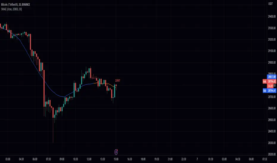
Simple Moving Average Extrapolation via Monte Carlo (SMAE)In this post, I will dive into my Moving Average Extrapolator, a tool that I created to help traders predict future price movements based on past data. I will discuss the underlying logic, its limitations, and the importance of accounting for delays in the moving average. The following code, my Moving Average Extrapolator, will serve as the basis for our discussion.
The Moving Average Extrapolator uses a simple moving average (SMA) to analyze past price movements and make predictions about future price movements. It uses a Monte Carlo simulation to generate possible future price movements based on historical probabilities.
Let's start by understanding the different components of the code:
The movement_probability function calculates the probability of green and red price movements, where green movements indicate an increase in price, and red movements indicate a decrease in price.
The monte function generates an array of potential price movements using a Monte Carlo simulation.
The sim function uses the generated Monte Carlo array to simulate potential future price movements based on the probabilities calculated earlier.
The draw_lines function draws lines connecting the current price to the extrapolated future price movements.
The extrapolate function calculates the extrapolated future price movements based on the provided source, length, and accuracy.
Limitations of My Moving Average Extrapolator:
Reliance on historical data: My Moving Average Extrapolator relies heavily on historical data to make future price predictions. This can be a limitation, as past performance does not guarantee future results. Market conditions can change, making the extrapolator less reliable in predicting future price movements.
Inherent randomness: The Monte Carlo simulation introduces an element of randomness in the extrapolator's predictions. While this can help in exploring various scenarios, it may not always accurately predict future price movements.
Delay in the moving average: Moving averages inherently have a delay, as they are based on past data. This delay can cause my Moving Average Extrapolator to be less accurate in predicting immediate price movements.
Accounting for Delays in the Moving Average:
It is essential to account for the delay in the moving average to improve the accuracy of my Moving Average Extrapolator. I have taken this into account by introducing a delay variable (delay) in the draw_lines function. The delay variable calculates the delay as half the moving average's length and adjusts the time axis accordingly.
This adjustment helps in reducing the lag in the extrapolator's predictions, making it more accurate and useful for traders. However, it is important to note that even with this adjustment, my Moving Average Extrapolator is still subject to the limitations discussed earlier.
Adding Custom Lookback Period to My Moving Average Extrapolator:
To enhance the functionality and adaptability of my Moving Average Extrapolator, I have implemented an option to set a custom lookback period. The lookback period determines how far back in the historical data the Moving Average Extrapolator should start its analysis.
To achieve this, I have included a method to obtain the current bar index and then calculate the starting bar index by subtracting the desired lookback period.
Here's how to implement the custom lookback period in the Moving Average Extrapolator:
Get the current bar index: I use the bar_index built-in variable to get the current bar index, which represents the current position in the historical data.
Set the start index: To set the start index, you can subtract the desired lookback period from the current bar index. In the code, I have defined a user-input number variable, which can be set to the desired lookback period. By default, it is set to 20800. The starting index for the Moving Average Extrapolator's analysis is calculated as bar_index - number.
Here's the relevant code snippet:
number = input.int(20800, "Bar Start")
And to conditionally run the calculations:
if bar_index > number
draw_lines(avg, extrapolate(close, length, 10), length, extrapolate)
By implementing this custom lookback period, users can easily adjust the starting point of the Moving Average Extrapolator based on their preferences and trading strategies. This allows for more flexibility and adaptability to different market scenarios and ensures that the Moving Average Extrapolator remains a valuable tool for traders.
Conclusion:
My Moving Average Extrapolator can be a valuable tool for traders looking to predict future price movements based on historical data. However, it is essential to understand its limitations and the need to account for the delay in the moving average. By considering these factors, traders can make better-informed decisions and use my Moving Average Extrapolator to complement their trading strategies effectively.
loxxfftLibrary "loxxfft"
This code is a library for performing Fast Fourier Transform (FFT) operations. FFT is an algorithm that can quickly compute the discrete Fourier transform (DFT) of a sequence. The library includes functions for performing FFTs on both real and complex data. It also includes functions for fast correlation and convolution, which are operations that can be performed efficiently using FFTs. Additionally, the library includes functions for fast sine and cosine transforms.
Reference:
www.alglib.net
fastfouriertransform(a, nn, inversefft)
Returns Fast Fourier Transform
Parameters:
a (float ) : float , An array of real and imaginary parts of the function values. The real part is stored at even indices, and the imaginary part is stored at odd indices.
nn (int) : int, The number of function values. It must be a power of two, but the algorithm does not validate this.
inversefft (bool) : bool, A boolean value that indicates the direction of the transformation. If True, it performs the inverse FFT; if False, it performs the direct FFT.
Returns: float , Modifies the input array a in-place, which means that the transformed data (the FFT result for direct transformation or the inverse FFT result for inverse transformation) will be stored in the same array a after the function execution. The transformed data will have real and imaginary parts interleaved, with the real parts at even indices and the imaginary parts at odd indices.
realfastfouriertransform(a, tnn, inversefft)
Returns Real Fast Fourier Transform
Parameters:
a (float ) : float , A float array containing the real-valued function samples.
tnn (int) : int, The number of function values (must be a power of 2, but the algorithm does not validate this condition).
inversefft (bool) : bool, A boolean flag that indicates the direction of the transformation (True for inverse, False for direct).
Returns: float , Modifies the input array a in-place, meaning that the transformed data (the FFT result for direct transformation or the inverse FFT result for inverse transformation) will be stored in the same array a after the function execution.
fastsinetransform(a, tnn, inversefst)
Returns Fast Discrete Sine Conversion
Parameters:
a (float ) : float , An array of real numbers representing the function values.
tnn (int) : int, Number of function values (must be a power of two, but the code doesn't validate this).
inversefst (bool) : bool, A boolean flag indicating the direction of the transformation. If True, it performs the inverse FST, and if False, it performs the direct FST.
Returns: float , The output is the transformed array 'a', which will contain the result of the transformation.
fastcosinetransform(a, tnn, inversefct)
Returns Fast Discrete Cosine Transform
Parameters:
a (float ) : float , This is a floating-point array representing the sequence of values (time-domain) that you want to transform. The function will perform the Fast Cosine Transform (FCT) or the inverse FCT on this input array, depending on the value of the inversefct parameter. The transformed result will also be stored in this same array, which means the function modifies the input array in-place.
tnn (int) : int, This is an integer value representing the number of data points in the input array a. It is used to determine the size of the input array and control the loops in the algorithm. Note that the size of the input array should be a power of 2 for the Fast Cosine Transform algorithm to work correctly.
inversefct (bool) : bool, This is a boolean value that controls whether the function performs the regular Fast Cosine Transform or the inverse FCT. If inversefct is set to true, the function will perform the inverse FCT, and if set to false, the regular FCT will be performed. The inverse FCT can be used to transform data back into its original form (time-domain) after the regular FCT has been applied.
Returns: float , The resulting transformed array is stored in the input array a. This means that the function modifies the input array in-place and does not return a new array.
fastconvolution(signal, signallen, response, negativelen, positivelen)
Convolution using FFT
Parameters:
signal (float ) : float , This is an array of real numbers representing the input signal that will be convolved with the response function. The elements are numbered from 0 to SignalLen-1.
signallen (int) : int, This is an integer representing the length of the input signal array. It specifies the number of elements in the signal array.
response (float ) : float , This is an array of real numbers representing the response function used for convolution. The response function consists of two parts: one corresponding to positive argument values and the other to negative argument values. Array elements with numbers from 0 to NegativeLen match the response values at points from -NegativeLen to 0, respectively. Array elements with numbers from NegativeLen+1 to NegativeLen+PositiveLen correspond to the response values in points from 1 to PositiveLen, respectively.
negativelen (int) : int, This is an integer representing the "negative length" of the response function. It indicates the number of elements in the response function array that correspond to negative argument values. Outside the range , the response function is considered zero.
positivelen (int) : int, This is an integer representing the "positive length" of the response function. It indicates the number of elements in the response function array that correspond to positive argument values. Similar to negativelen, outside the range , the response function is considered zero.
Returns: float , The resulting convolved values are stored back in the input signal array.
fastcorrelation(signal, signallen, pattern, patternlen)
Returns Correlation using FFT
Parameters:
signal (float ) : float ,This is an array of real numbers representing the signal to be correlated with the pattern. The elements are numbered from 0 to SignalLen-1.
signallen (int) : int, This is an integer representing the length of the input signal array.
pattern (float ) : float , This is an array of real numbers representing the pattern to be correlated with the signal. The elements are numbered from 0 to PatternLen-1.
patternlen (int) : int, This is an integer representing the length of the pattern array.
Returns: float , The signal array containing the correlation values at points from 0 to SignalLen-1.
tworealffts(a1, a2, a, b, tn)
Returns Fast Fourier Transform of Two Real Functions
Parameters:
a1 (float ) : float , An array of real numbers, representing the values of the first function.
a2 (float ) : float , An array of real numbers, representing the values of the second function.
a (float ) : float , An output array to store the Fourier transform of the first function.
b (float ) : float , An output array to store the Fourier transform of the second function.
tn (int) : float , An integer representing the number of function values. It must be a power of two, but the algorithm doesn't validate this condition.
Returns: float , The a and b arrays will contain the Fourier transform of the first and second functions, respectively. Note that the function overwrites the input arrays a and b.
█ Detailed explaination of each function
Fast Fourier Transform
The fastfouriertransform() function takes three input parameters:
1. a: An array of real and imaginary parts of the function values. The real part is stored at even indices, and the imaginary part is stored at odd indices.
2. nn: The number of function values. It must be a power of two, but the algorithm does not validate this.
3. inversefft: A boolean value that indicates the direction of the transformation. If True, it performs the inverse FFT; if False, it performs the direct FFT.
The function performs the FFT using the Cooley-Tukey algorithm, which is an efficient algorithm for computing the discrete Fourier transform (DFT) and its inverse. The Cooley-Tukey algorithm recursively breaks down the DFT of a sequence into smaller DFTs of subsequences, leading to a significant reduction in computational complexity. The algorithm's time complexity is O(n log n), where n is the number of samples.
The fastfouriertransform() function first initializes variables and determines the direction of the transformation based on the inversefft parameter. If inversefft is True, the isign variable is set to -1; otherwise, it is set to 1.
Next, the function performs the bit-reversal operation. This is a necessary step before calculating the FFT, as it rearranges the input data in a specific order required by the Cooley-Tukey algorithm. The bit-reversal is performed using a loop that iterates through the nn samples, swapping the data elements according to their bit-reversed index.
After the bit-reversal operation, the function iteratively computes the FFT using the Cooley-Tukey algorithm. It performs calculations in a loop that goes through different stages, doubling the size of the sub-FFT at each stage. Within each stage, the Cooley-Tukey algorithm calculates the butterfly operations, which are mathematical operations that combine the results of smaller DFTs into the final DFT. The butterfly operations involve complex number multiplication and addition, updating the input array a with the computed values.
The loop also calculates the twiddle factors, which are complex exponential factors used in the butterfly operations. The twiddle factors are calculated using trigonometric functions, such as sine and cosine, based on the angle theta. The variables wpr, wpi, wr, and wi are used to store intermediate values of the twiddle factors, which are updated in each iteration of the loop.
Finally, if the inversefft parameter is True, the function divides the result by the number of samples nn to obtain the correct inverse FFT result. This normalization step is performed using a loop that iterates through the array a and divides each element by nn.
In summary, the fastfouriertransform() function is an implementation of the Cooley-Tukey FFT algorithm, which is an efficient algorithm for computing the DFT and its inverse. This FFT library can be used for a variety of applications, such as signal processing, image processing, audio processing, and more.
Feal Fast Fourier Transform
The realfastfouriertransform() function performs a fast Fourier transform (FFT) specifically for real-valued functions. The FFT is an efficient algorithm used to compute the discrete Fourier transform (DFT) and its inverse, which are fundamental tools in signal processing, image processing, and other related fields.
This function takes three input parameters:
1. a - A float array containing the real-valued function samples.
2. tnn - The number of function values (must be a power of 2, but the algorithm does not validate this condition).
3. inversefft - A boolean flag that indicates the direction of the transformation (True for inverse, False for direct).
The function modifies the input array a in-place, meaning that the transformed data (the FFT result for direct transformation or the inverse FFT result for inverse transformation) will be stored in the same array a after the function execution.
The algorithm uses a combination of complex-to-complex FFT and additional transformations specific to real-valued data to optimize the computation. It takes into account the symmetry properties of the real-valued input data to reduce the computational complexity.
Here's a detailed walkthrough of the algorithm:
1. Depending on the inversefft flag, the initial values for ttheta, c1, and c2 are determined. These values are used for the initial data preprocessing and post-processing steps specific to the real-valued FFT.
2. The preprocessing step computes the initial real and imaginary parts of the data using a combination of sine and cosine terms with the input data. This step effectively converts the real-valued input data into complex-valued data suitable for the complex-to-complex FFT.
3. The complex-to-complex FFT is then performed on the preprocessed complex data. This involves bit-reversal reordering, followed by the Cooley-Tukey radix-2 decimation-in-time algorithm. This part of the code is similar to the fastfouriertransform() function you provided earlier.
4. After the complex-to-complex FFT, a post-processing step is performed to obtain the final real-valued output data. This involves updating the real and imaginary parts of the transformed data using sine and cosine terms, as well as the values c1 and c2.
5. Finally, if the inversefft flag is True, the output data is divided by the number of samples (nn) to obtain the inverse DFT.
The function does not return a value explicitly. Instead, the transformed data is stored in the input array a. After the function execution, you can access the transformed data in the a array, which will have the real part at even indices and the imaginary part at odd indices.
Fast Sine Transform
This code defines a function called fastsinetransform that performs a Fast Discrete Sine Transform (FST) on an array of real numbers. The function takes three input parameters:
1. a (float array): An array of real numbers representing the function values.
2. tnn (int): Number of function values (must be a power of two, but the code doesn't validate this).
3. inversefst (bool): A boolean flag indicating the direction of the transformation. If True, it performs the inverse FST, and if False, it performs the direct FST.
The output is the transformed array 'a', which will contain the result of the transformation.
The code starts by initializing several variables, including trigonometric constants for the sine transform. It then sets the first value of the array 'a' to 0 and calculates the initial values of 'y1' and 'y2', which are used to update the input array 'a' in the following loop.
The first loop (with index 'jx') iterates from 2 to (tm + 1), where 'tm' is half of the number of input samples 'tnn'. This loop is responsible for calculating the initial sine transform of the input data.
The second loop (with index 'ii') is a bit-reversal loop. It reorders the elements in the array 'a' based on the bit-reversed indices of the original order.
The third loop (with index 'ii') iterates while 'n' is greater than 'mmax', which starts at 2 and doubles each iteration. This loop performs the actual Fast Discrete Sine Transform. It calculates the sine transform using the Danielson-Lanczos lemma, which is a divide-and-conquer strategy for calculating Discrete Fourier Transforms (DFTs) efficiently.
The fourth loop (with index 'ix') is responsible for the final phase adjustments needed for the sine transform, updating the array 'a' accordingly.
The fifth loop (with index 'jj') updates the array 'a' one more time by dividing each element by 2 and calculating the sum of the even-indexed elements.
Finally, if the 'inversefst' flag is True, the code scales the transformed data by a factor of 2/tnn to get the inverse Fast Sine Transform.
In summary, the code performs a Fast Discrete Sine Transform on an input array of real numbers, either in the direct or inverse direction, and returns the transformed array. The algorithm is based on the Danielson-Lanczos lemma and uses a divide-and-conquer strategy for efficient computation.
Fast Cosine Transform
This code defines a function called fastcosinetransform that takes three parameters: a floating-point array a, an integer tnn, and a boolean inversefct. The function calculates the Fast Cosine Transform (FCT) or the inverse FCT of the input array, depending on the value of the inversefct parameter.
The Fast Cosine Transform is an algorithm that converts a sequence of values (time-domain) into a frequency domain representation. It is closely related to the Fast Fourier Transform (FFT) and can be used in various applications, such as signal processing and image compression.
Here's a detailed explanation of the code:
1. The function starts by initializing a number of variables, including counters, intermediate values, and constants.
2. The initial steps of the algorithm are performed. This includes calculating some trigonometric values and updating the input array a with the help of intermediate variables.
3. The code then enters a loop (from jx = 2 to tnn / 2). Within this loop, the algorithm computes and updates the elements of the input array a.
4. After the loop, the function prepares some variables for the next stage of the algorithm.
5. The next part of the algorithm is a series of nested loops that perform the bit-reversal permutation and apply the FCT to the input array a.
6. The code then calculates some additional trigonometric values, which are used in the next loop.
7. The following loop (from ix = 2 to tnn / 4 + 1) computes and updates the elements of the input array a using the previously calculated trigonometric values.
8. The input array a is further updated with the final calculations.
9. In the last loop (from j = 4 to tnn), the algorithm computes and updates the sum of elements in the input array a.
10. Finally, if the inversefct parameter is set to true, the function scales the input array a to obtain the inverse FCT.
The resulting transformed array is stored in the input array a. This means that the function modifies the input array in-place and does not return a new array.
Fast Convolution
This code defines a function called fastconvolution that performs the convolution of a given signal with a response function using the Fast Fourier Transform (FFT) technique. Convolution is a mathematical operation used in signal processing to combine two signals, producing a third signal representing how the shape of one signal is modified by the other.
The fastconvolution function takes the following input parameters:
1. float signal: This is an array of real numbers representing the input signal that will be convolved with the response function. The elements are numbered from 0 to SignalLen-1.
2. int signallen: This is an integer representing the length of the input signal array. It specifies the number of elements in the signal array.
3. float response: This is an array of real numbers representing the response function used for convolution. The response function consists of two parts: one corresponding to positive argument values and the other to negative argument values. Array elements with numbers from 0 to NegativeLen match the response values at points from -NegativeLen to 0, respectively. Array elements with numbers from NegativeLen+1 to NegativeLen+PositiveLen correspond to the response values in points from 1 to PositiveLen, respectively.
4. int negativelen: This is an integer representing the "negative length" of the response function. It indicates the number of elements in the response function array that correspond to negative argument values. Outside the range , the response function is considered zero.
5. int positivelen: This is an integer representing the "positive length" of the response function. It indicates the number of elements in the response function array that correspond to positive argument values. Similar to negativelen, outside the range , the response function is considered zero.
The function works by:
1. Calculating the length nl of the arrays used for FFT, ensuring it's a power of 2 and large enough to hold the signal and response.
2. Creating two new arrays, a1 and a2, of length nl and initializing them with the input signal and response function, respectively.
3. Applying the forward FFT (realfastfouriertransform) to both arrays, a1 and a2.
4. Performing element-wise multiplication of the FFT results in the frequency domain.
5. Applying the inverse FFT (realfastfouriertransform) to the multiplied results in a1.
6. Updating the original signal array with the convolution result, which is stored in the a1 array.
The result of the convolution is stored in the input signal array at the function exit.
Fast Correlation
This code defines a function called fastcorrelation that computes the correlation between a signal and a pattern using the Fast Fourier Transform (FFT) method. The function takes four input arguments and modifies the input signal array to store the correlation values.
Input arguments:
1. float signal: This is an array of real numbers representing the signal to be correlated with the pattern. The elements are numbered from 0 to SignalLen-1.
2. int signallen: This is an integer representing the length of the input signal array.
3. float pattern: This is an array of real numbers representing the pattern to be correlated with the signal. The elements are numbered from 0 to PatternLen-1.
4. int patternlen: This is an integer representing the length of the pattern array.
The function performs the following steps:
1. Calculate the required size nl for the FFT by finding the smallest power of 2 that is greater than or equal to the sum of the lengths of the signal and the pattern.
2. Create two new arrays a1 and a2 with the length nl and initialize them to 0.
3. Copy the signal array into a1 and pad it with zeros up to the length nl.
4. Copy the pattern array into a2 and pad it with zeros up to the length nl.
5. Compute the FFT of both a1 and a2.
6. Perform element-wise multiplication of the frequency-domain representation of a1 and the complex conjugate of the frequency-domain representation of a2.
7. Compute the inverse FFT of the result obtained in step 6.
8. Store the resulting correlation values in the original signal array.
At the end of the function, the signal array contains the correlation values at points from 0 to SignalLen-1.
Fast Fourier Transform of Two Real Functions
This code defines a function called tworealffts that computes the Fast Fourier Transform (FFT) of two real-valued functions (a1 and a2) using a Cooley-Tukey-based radix-2 Decimation in Time (DIT) algorithm. The FFT is a widely used algorithm for computing the discrete Fourier transform (DFT) and its inverse.
Input parameters:
1. float a1: an array of real numbers, representing the values of the first function.
2. float a2: an array of real numbers, representing the values of the second function.
3. float a: an output array to store the Fourier transform of the first function.
4. float b: an output array to store the Fourier transform of the second function.
5. int tn: an integer representing the number of function values. It must be a power of two, but the algorithm doesn't validate this condition.
The function performs the following steps:
1. Combine the two input arrays, a1 and a2, into a single array a by interleaving their elements.
2. Perform a 1D FFT on the combined array a using the radix-2 DIT algorithm.
3. Separate the FFT results of the two input functions from the combined array a and store them in output arrays a and b.
Here is a detailed breakdown of the radix-2 DIT algorithm used in this code:
1. Bit-reverse the order of the elements in the combined array a.
2. Initialize the loop variables mmax, istep, and theta.
3. Enter the main loop that iterates through different stages of the FFT.
a. Compute the sine and cosine values for the current stage using the theta variable.
b. Initialize the loop variables wr and wi for the current stage.
c. Enter the inner loop that iterates through the butterfly operations within each stage.
i. Perform the butterfly operation on the elements of array a.
ii. Update the loop variables wr and wi for the next butterfly operation.
d. Update the loop variables mmax, istep, and theta for the next stage.
4. Separate the FFT results of the two input functions from the combined array a and store them in output arrays a and b.
At the end of the function, the a and b arrays will contain the Fourier transform of the first and second functions, respectively. Note that the function overwrites the input arrays a and b.
█ Example scripts using functions contained in loxxfft
Real-Fast Fourier Transform of Price w/ Linear Regression
Real-Fast Fourier Transform of Price Oscillator
Normalized, Variety, Fast Fourier Transform Explorer
Variety RSI of Fast Discrete Cosine Transform
STD-Stepped Fast Cosine Transform Moving Average
TR_HighLow_LibLibrary "TR_HighLow_Lib"
TODO: add library description here
ShowLabel(_Text, _X, _Y, _Style, _Size, _Yloc, _Color)
TODO: Function to display labels
Parameters:
_Text : TODO: text (series string) Label text.
_X : TODO: x (series int) Bar index.
_Y : TODO: y (series int/float) Price of the label position.
_Style : TODO: style (series string) Label style.
_Size : TODO: size (series string) Label size.
_Yloc : TODO: yloc (series string) Possible values are yloc.price, yloc.abovebar, yloc.belowbar.
_Color : TODO: color (series color) Color of the label border and arrow
Returns: TODO: No return values
GetColor(_Index)
TODO: Function to take out 12 colors in order
Parameters:
_Index : TODO: color number.
Returns: TODO: color code
Tbl_position(_Pos)
TODO: Table display position function
Parameters:
_Pos : TODO: position.
Returns: TODO: Table position
DeleteLine()
TODO: Delete Line
Parameters:
: TODO: No parameter
Returns: TODO: No return value
DeleteLabel()
TODO: Delete Label
Parameters:
: TODO: No parameter
Returns: TODO: No return value
ZigZag(_a_PHiLo, _a_IHiLo, _a_FHiLo, _a_DHiLo, _Histories, _Provisional_PHiLo, _Provisional_IHiLo, _Color1, _Width1, _Color2, _Width2, _ShowLabel, _ShowHighLowBar, _HighLowBarWidth, _HighLow_LabelSize)
TODO: Draw a zig-zag line.
Parameters:
_a_PHiLo : TODO: High-Low price array
_a_IHiLo : TODO: High-Low INDEX array
_a_FHiLo : TODO: High-Low flag array sequence 1:High 2:Low
_a_DHiLo : TODO: High-Low Price Differential Array
_Histories : TODO: Array size (High-Low length)
_Provisional_PHiLo : TODO: Provisional High-Low Price
_Provisional_IHiLo : TODO: Provisional High-Low INDEX
_Color1 : TODO: Normal High-Low color
_Width1 : TODO: Normal High-Low width
_Color2 : TODO: Provisional High-Low color
_Width2 : TODO: Provisional High-Low width
_ShowLabel : TODO: Label display flag True: Displayed False: Not displayed
_ShowHighLowBar : TODO: High-Low bar display flag True:Show False:Hide
_HighLowBarWidth : TODO: High-Low bar width
_HighLow_LabelSize : TODO: Label Size
Returns: TODO: No return value
TrendLine(_a_PHiLo, _a_IHiLo, _Histories, _MultiLine, _StartWidth, _EndWidth, _IncreWidth, _StartTrans, _EndTrans, _IncreTrans, _ColorMode, _Color1_1, _Color1_2, _Color2_1, _Color2_2, _Top_High, _Top_Low, _Bottom_High, _Bottom_Low)
TODO: Draw a Trend Line
Parameters:
_a_PHiLo : TODO: High-Low price array
_a_IHiLo : TODO: High-Low INDEX array
_Histories : TODO: Array size (High-Low length)
_MultiLine : TODO: Draw a multiple Line.
_StartWidth : TODO: Line width start value
_EndWidth : TODO: Line width end value
_IncreWidth : TODO: Line width increment value
_StartTrans : TODO: Transparent rate start value
_EndTrans : TODO: Transparent rate finally
_IncreTrans : TODO: Transparent rate increase value
_ColorMode : TODO: 0:Nomal 1:Gradation
_Color1_1 : TODO: Gradation Color 1_1
_Color1_2 : TODO: Gradation Color 1_2
_Color2_1 : TODO: Gradation Color 2_1
_Color2_2 : TODO: Gradation Color 2_2
_Top_High : TODO: _Top_High Value for Gradation
_Top_Low : TODO: _Top_Low Value for Gradation
_Bottom_High : TODO: _Bottom_High Value for Gradation
_Bottom_Low : TODO: _Bottom_Low Value for Gradation
Returns: TODO: No return value
Fibonacci(_a_Fibonacci, _a_PHiLo, _Provisional_PHiLo, _Index, _FrontMargin, _BackMargin)
TODO: Draw a Fibonacci line
Parameters:
_a_Fibonacci : TODO: Fibonacci Percentage Array
_a_PHiLo : TODO: High-Low price array
_Provisional_PHiLo : TODO: Provisional High-Low price (when _Index is 0)
_Index : TODO: Where to draw the Fibonacci line
_FrontMargin : TODO: Fibonacci line front-margin
_BackMargin : TODO: Fibonacci line back-margin
Returns: TODO: No return value
Fibonacci(_a_Fibonacci, _a_PHiLo, _Provisional_PHiLo, _Index1, _FrontMargin1, _BackMargin1, _Transparent1, _Index2, _FrontMargin2, _BackMargin2, _Transparent2)
TODO: Draw a Fibonacci line
Parameters:
_a_Fibonacci : TODO: Fibonacci Percentage Array
_a_PHiLo : TODO: High-Low price array
_Provisional_PHiLo : TODO: Provisional High-Low price (when _Index is 0)
_Index1 : TODO: Where to draw the Fibonacci line 1
_FrontMargin1 : TODO: Fibonacci line front-margin 1
_BackMargin1 : TODO: Fibonacci line back-margin 1
_Transparent1 : TODO: Transparent rate 1
_Index2 : TODO: Where to draw the Fibonacci line 2
_FrontMargin2 : TODO: Fibonacci line front-margin 2
_BackMargin2 : TODO: Fibonacci line back-margin 2
_Transparent2 : TODO: Transparent rate 2
Returns: TODO: No return value
High_Low_Judgment(_Length, _Extension, _Difference)
TODO: Judges High-Low
Parameters:
_Length : TODO: High-Low Confirmation Length
_Extension : TODO: Length of extension when the difference did not open
_Difference : TODO: Difference size
Returns: TODO: _HiLo=High-Low flag 0:Neither high nor low、1:High、2:Low、3:High-Low
_PHi=high price、_PLo=low price、_IHi=High Price Index、_ILo=Low Price Index、
_Cnt=count、_ECnt=Extension count、
_DiffHi=Difference from Start(High)、_DiffLo=Difference from Start(Low)、
_StartHi=Start value(High)、_StartLo=Start value(Low)
High_Low_Data_AddedAndUpdated(_HiLo, _Histories, _PHi, _PLo, _IHi, _ILo, _DiffHi, _DiffLo, _a_PHiLo, _a_IHiLo, _a_FHiLo, _a_DHiLo)
TODO: Adds and updates High-Low related arrays from given parameters
Parameters:
_HiLo : TODO: High-Low flag
_Histories : TODO: Array size (High-Low length)
_PHi : TODO: Price Hi
_PLo : TODO: Price Lo
_IHi : TODO: Index Hi
_ILo : TODO: Index Lo
_DiffHi : TODO: Difference in High
_DiffLo : TODO: Difference in Low
_a_PHiLo : TODO: High-Low price array
_a_IHiLo : TODO: High-Low INDEX array
_a_FHiLo : TODO: High-Low flag array 1:High 2:Low
_a_DHiLo : TODO: High-Low Price Differential Array
Returns: TODO: _PHiLo price array、_IHiLo indexed array、_FHiLo flag array、_DHiLo price-matching array、
Provisional_PHiLo Provisional price、Provisional_IHiLo 暫定インデックス
High_Low(_a_PHiLo, _a_IHiLo, _a_FHiLo, _a_DHiLo, _a_Fibonacci, _Length, _Extension, _Difference, _Histories, _ShowZigZag, _ZigZagColor1, _ZigZagWidth1, _ZigZagColor2, _ZigZagWidth2, _ShowZigZagLabel, _ShowHighLowBar, _ShowTrendLine, _TrendMultiLine, _TrendStartWidth, _TrendEndWidth, _TrendIncreWidth, _TrendStartTrans, _TrendEndTrans, _TrendIncreTrans, _TrendColorMode, _TrendColor1_1, _TrendColor1_2, _TrendColor2_1, _TrendColor2_2, _ShowFibonacci1, _FibIndex1, _FibFrontMargin1, _FibBackMargin1, _FibTransparent1, _ShowFibonacci2, _FibIndex2, _FibFrontMargin2, _FibBackMargin2, _FibTransparent2, _ShowInfoTable1, _TablePosition1, _ShowInfoTable2, _TablePosition2)
TODO: Draw the contents of the High-Low array.
Parameters:
_a_PHiLo : TODO: High-Low price array
_a_IHiLo : TODO: High-Low INDEX array
_a_FHiLo : TODO: High-Low flag sequence 1:High 2:Low
_a_DHiLo : TODO: High-Low Price Differential Array
_a_Fibonacci : TODO: Fibonacci Gnar Matching
_Length : TODO: Length of confirmation
_Extension : TODO: Extension Length of extension when the difference did not open
_Difference : TODO: Difference size
_Histories : TODO: High-Low Length
_ShowZigZag : TODO: ZigZag Display
_ZigZagColor1 : TODO: Colors of ZigZag1
_ZigZagWidth1 : TODO: Width of ZigZag1
_ZigZagColor2 : TODO: Colors of ZigZag2
_ZigZagWidth2 : TODO: Width of ZigZag2
_ShowZigZagLabel : TODO: ZigZagLabel Display
_ShowHighLowBar : TODO: High-Low Bar Display
_ShowTrendLine : TODO: Trend Line Display
_TrendMultiLine : TODO: Trend Multi Line Display
_TrendStartWidth : TODO: Line width start value
_TrendEndWidth : TODO: Line width end value
_TrendIncreWidth : TODO: Line width increment value
_TrendStartTrans : TODO: Starting transmittance value
_TrendEndTrans : TODO: Transmittance End Value
_TrendIncreTrans : TODO: Increased transmittance value
_TrendColorMode : TODO: color mode
_TrendColor1_1 : TODO: Trend Color 1_1
_TrendColor1_2 : TODO: Trend Color 1_2
_TrendColor2_1 : TODO: Trend Color 2_1
_TrendColor2_2 : TODO: Trend Color 2_2
_ShowFibonacci1 : TODO: Fibonacci1 Display
_FibIndex1 : TODO: Fibonacci1 Index No.
_FibFrontMargin1 : TODO: Fibonacci1 Front margin
_FibBackMargin1 : TODO: Fibonacci1 Back Margin
_FibTransparent1 : TODO: Fibonacci1 Transmittance
_ShowFibonacci2 : TODO: Fibonacci2 Display
_FibIndex2 : TODO: Fibonacci2 Index No.
_FibFrontMargin2 : TODO: Fibonacci2 Front margin
_FibBackMargin2 : TODO: Fibonacci2 Back Margin
_FibTransparent2 : TODO: Fibonacci2 Transmittance
_ShowInfoTable1 : TODO: InfoTable1 Display
_TablePosition1 : TODO: InfoTable1 position
_ShowInfoTable2 : TODO: InfoTable2 Display
_TablePosition2 : TODO: InfoTable2 position
Returns: TODO: 無し

TR_HighLowLibrary "TR_HighLow"
TODO: add library description here
ShowLabel(_Text, _X, _Y, _Style, _Size, _Yloc, _Color)
TODO: Function to display labels
Parameters:
_Text : TODO: text (series string) Label text.
_X : TODO: x (series int) Bar index.
_Y : TODO: y (series int/float) Price of the label position.
_Style : TODO: style (series string) Label style.
_Size : TODO: size (series string) Label size.
_Yloc : TODO: yloc (series string) Possible values are yloc.price, yloc.abovebar, yloc.belowbar.
_Color : TODO: color (series color) Color of the label border and arrow
Returns: TODO: No return values
GetColor(_Index)
TODO: Function to take out 12 colors in order
Parameters:
_Index : TODO: color number.
Returns: TODO: color code
Tbl_position(_Pos)
TODO: Table display position function
Parameters:
_Pos : TODO: position.
Returns: TODO: Table position
DeleteLine()
TODO: Delete Line
Parameters:
: TODO: No parameter
Returns: TODO: No return value
DeleteLabel()
TODO: Delete Label
Parameters:
: TODO: No parameter
Returns: TODO: No return value
ZigZag(_a_PHiLo, _a_IHiLo, _a_FHiLo, _a_DHiLo, _Histories, _Provisional_PHiLo, _Provisional_IHiLo, _Color1, _Width1, _Color2, _Width2, _ShowLabel, _ShowHighLowBar, _HighLowBarWidth, _HighLow_LabelSize)
TODO: Draw a zig-zag line.
Parameters:
_a_PHiLo : TODO: High-Low price array
_a_IHiLo : TODO: High-Low INDEX array
_a_FHiLo : TODO: High-Low flag array sequence 1:High 2:Low
_a_DHiLo : TODO: High-Low Price Differential Array
_Histories : TODO: Array size (High-Low length)
_Provisional_PHiLo : TODO: Provisional High-Low Price
_Provisional_IHiLo : TODO: Provisional High-Low INDEX
_Color1 : TODO: Normal High-Low color
_Width1 : TODO: Normal High-Low width
_Color2 : TODO: Provisional High-Low color
_Width2 : TODO: Provisional High-Low width
_ShowLabel : TODO: Label display flag True: Displayed False: Not displayed
_ShowHighLowBar : TODO: High-Low bar display flag True:Show False:Hide
_HighLowBarWidth : TODO: High-Low bar width
_HighLow_LabelSize : TODO: Label Size
Returns: TODO: No return value
TrendLine(_a_PHiLo, _a_IHiLo, _Histories, _MultiLine, _StartWidth, _EndWidth, _IncreWidth, _StartTrans, _EndTrans, _IncreTrans, _ColorMode, _Color1_1, _Color1_2, _Color2_1, _Color2_2, _Top_High, _Top_Low, _Bottom_High, _Bottom_Low)
TODO: Draw a Trend Line
Parameters:
_a_PHiLo : TODO: High-Low price array
_a_IHiLo : TODO: High-Low INDEX array
_Histories : TODO: Array size (High-Low length)
_MultiLine : TODO: Draw a multiple Line.
_StartWidth : TODO: Line width start value
_EndWidth : TODO: Line width end value
_IncreWidth : TODO: Line width increment value
_StartTrans : TODO: Transparent rate start value
_EndTrans : TODO: Transparent rate finally
_IncreTrans : TODO: Transparent rate increase value
_ColorMode : TODO: 0:Nomal 1:Gradation
_Color1_1 : TODO: Gradation Color 1_1
_Color1_2 : TODO: Gradation Color 1_2
_Color2_1 : TODO: Gradation Color 2_1
_Color2_2 : TODO: Gradation Color 2_2
_Top_High : TODO: _Top_High Value for Gradation
_Top_Low : TODO: _Top_Low Value for Gradation
_Bottom_High : TODO: _Bottom_High Value for Gradation
_Bottom_Low : TODO: _Bottom_Low Value for Gradation
Returns: TODO: No return value
Fibonacci(_a_Fibonacci, _a_PHiLo, _Provisional_PHiLo, _Index, _FrontMargin, _BackMargin)
TODO: Draw a Fibonacci line
Parameters:
_a_Fibonacci : TODO: Fibonacci Percentage Array
_a_PHiLo : TODO: High-Low price array
_Provisional_PHiLo : TODO: Provisional High-Low price (when _Index is 0)
_Index : TODO: Where to draw the Fibonacci line
_FrontMargin : TODO: Fibonacci line front-margin
_BackMargin : TODO: Fibonacci line back-margin
Returns: TODO: No return value
Fibonacci(_a_Fibonacci, _a_PHiLo, _Provisional_PHiLo, _Index1, _FrontMargin1, _BackMargin1, _Transparent1, _Index2, _FrontMargin2, _BackMargin2, _Transparent2)
TODO: Draw a Fibonacci line
Parameters:
_a_Fibonacci : TODO: Fibonacci Percentage Array
_a_PHiLo : TODO: High-Low price array
_Provisional_PHiLo : TODO: Provisional High-Low price (when _Index is 0)
_Index1 : TODO: Where to draw the Fibonacci line 1
_FrontMargin1 : TODO: Fibonacci line front-margin 1
_BackMargin1 : TODO: Fibonacci line back-margin 1
_Transparent1 : TODO: Transparent rate 1
_Index2 : TODO: Where to draw the Fibonacci line 2
_FrontMargin2 : TODO: Fibonacci line front-margin 2
_BackMargin2 : TODO: Fibonacci line back-margin 2
_Transparent2 : TODO: Transparent rate 2
Returns: TODO: No return value
High_Low_Judgment(_Length, _Extension, _Difference)
TODO: Judges High-Low
Parameters:
_Length : TODO: High-Low Confirmation Length
_Extension : TODO: Length of extension when the difference did not open
_Difference : TODO: Difference size
Returns: TODO: _HiLo=High-Low flag 0:Neither high nor low、1:High、2:Low、3:High-Low
_PHi=high price、_PLo=low price、_IHi=High Price Index、_ILo=Low Price Index、
_Cnt=count、_ECnt=Extension count、
_DiffHi=Difference from Start(High)、_DiffLo=Difference from Start(Low)、
_StartHi=Start value(High)、_StartLo=Start value(Low)
High_Low_Data_AddedAndUpdated(_HiLo, _Histories, _PHi, _PLo, _IHi, _ILo, _DiffHi, _DiffLo, _a_PHiLo, _a_IHiLo, _a_FHiLo, _a_DHiLo)
TODO: Adds and updates High-Low related arrays from given parameters
Parameters:
_HiLo : TODO: High-Low flag
_Histories : TODO: Array size (High-Low length)
_PHi : TODO: Price Hi
_PLo : TODO: Price Lo
_IHi : TODO: Index Hi
_ILo : TODO: Index Lo
_DiffHi : TODO: Difference in High
_DiffLo : TODO: Difference in Low
_a_PHiLo : TODO: High-Low price array
_a_IHiLo : TODO: High-Low INDEX array
_a_FHiLo : TODO: High-Low flag array 1:High 2:Low
_a_DHiLo : TODO: High-Low Price Differential Array
Returns: TODO: _PHiLo price array、_IHiLo indexed array、_FHiLo flag array、_DHiLo price-matching array、
Provisional_PHiLo Provisional price、Provisional_IHiLo 暫定インデックス
High_Low(_a_PHiLo, _a_IHiLo, _a_FHiLo, _a_DHiLo, _a_Fibonacci, _Length, _Extension, _Difference, _Histories, _ShowZigZag, _ZigZagColor1, _ZigZagWidth1, _ZigZagColor2, _ZigZagWidth2, _ShowZigZagLabel, _ShowHighLowBar, _ShowTrendLine, _TrendMultiLine, _TrendStartWidth, _TrendEndWidth, _TrendIncreWidth, _TrendStartTrans, _TrendEndTrans, _TrendIncreTrans, _TrendColorMode, _TrendColor1_1, _TrendColor1_2, _TrendColor2_1, _TrendColor2_2, _ShowFibonacci1, _FibIndex1, _FibFrontMargin1, _FibBackMargin1, _FibTransparent1, _ShowFibonacci2, _FibIndex2, _FibFrontMargin2, _FibBackMargin2, _FibTransparent2, _ShowInfoTable1, _TablePosition1, _ShowInfoTable2, _TablePosition2)
TODO: Draw the contents of the High-Low array.
Parameters:
_a_PHiLo : TODO: High-Low price array
_a_IHiLo : TODO: High-Low INDEX array
_a_FHiLo : TODO: High-Low flag sequence 1:High 2:Low
_a_DHiLo : TODO: High-Low Price Differential Array
_a_Fibonacci : TODO: Fibonacci Gnar Matching
_Length : TODO: Length of confirmation
_Extension : TODO: Extension Length of extension when the difference did not open
_Difference : TODO: Difference size
_Histories : TODO: High-Low Length
_ShowZigZag : TODO: ZigZag Display
_ZigZagColor1 : TODO: Colors of ZigZag1
_ZigZagWidth1 : TODO: Width of ZigZag1
_ZigZagColor2 : TODO: Colors of ZigZag2
_ZigZagWidth2 : TODO: Width of ZigZag2
_ShowZigZagLabel : TODO: ZigZagLabel Display
_ShowHighLowBar : TODO: High-Low Bar Display
_ShowTrendLine : TODO: Trend Line Display
_TrendMultiLine : TODO: Trend Multi Line Display
_TrendStartWidth : TODO: Line width start value
_TrendEndWidth : TODO: Line width end value
_TrendIncreWidth : TODO: Line width increment value
_TrendStartTrans : TODO: Starting transmittance value
_TrendEndTrans : TODO: Transmittance End Value
_TrendIncreTrans : TODO: Increased transmittance value
_TrendColorMode : TODO: color mode
_TrendColor1_1 : TODO: Trend Color 1_1
_TrendColor1_2 : TODO: Trend Color 1_2
_TrendColor2_1 : TODO: Trend Color 2_1
_TrendColor2_2 : TODO: Trend Color 2_2
_ShowFibonacci1 : TODO: Fibonacci1 Display
_FibIndex1 : TODO: Fibonacci1 Index No.
_FibFrontMargin1 : TODO: Fibonacci1 Front margin
_FibBackMargin1 : TODO: Fibonacci1 Back Margin
_FibTransparent1 : TODO: Fibonacci1 Transmittance
_ShowFibonacci2 : TODO: Fibonacci2 Display
_FibIndex2 : TODO: Fibonacci2 Index No.
_FibFrontMargin2 : TODO: Fibonacci2 Front margin
_FibBackMargin2 : TODO: Fibonacci2 Back Margin
_FibTransparent2 : TODO: Fibonacci2 Transmittance
_ShowInfoTable1 : TODO: InfoTable1 Display
_TablePosition1 : TODO: InfoTable1 position
_ShowInfoTable2 : TODO: InfoTable2 Display
_TablePosition2 : TODO: InfoTable2 position
Returns: TODO: 無し

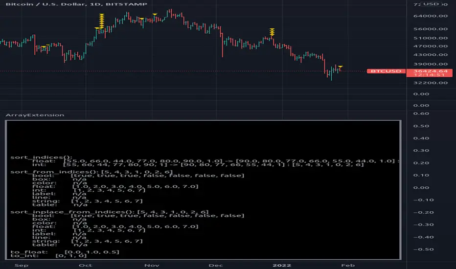
ArrayExtensionLibrary "ArrayExtension"
Functions to extend Arrays.
index_2d_to_1d(dimension_x, dimension_y, index_x, index_y) returns the flatened one dimension index of a two dimension array.
Parameters:
dimension_x : int, dimension of X.
dimension_y : int, dimension of Y.
index_x : int, index of X.
index_y : int, index of Y.
Returns: int, index in 1 dimension
index_3d_to_1d(dimension_x, dimension_y, dimension_z, index_x, index_y, index_z) returns the flatened one dimension index of a three dimension array.
Parameters:
dimension_x : int, dimension of X.
dimension_y : int, dimension of Y.
dimension_z : int, dimension of Z.
index_x : int, index of X.
index_y : int, index of Y.
index_z : int, index of Z.
Returns: int, index in 1 dimension
down_sample(sample, new_size) Down samples a array to a specified size.
Parameters:
sample : float array, array with source data.
new_size : new size of down sampled array.
Returns: float array with down sampled data.
sort_indices_float(sample, order) Sorts array and returns a extra array with sorting indices.
Parameters:
sample : float array with values to be sorted.
order : string, default='forward', options='forward', 'backward'.
Returns: _indices int array with indices.
_ordered float array with ordered values.
sort_indices_int(sample, order) Sorts array and returns a extra array with sorting indices.
Parameters:
sample : int array with values to be sorted.
order : string, default='forward', options='forward', 'backward'.
Returns: _indices int array with indices.
_ordered float array with ordered values.
sort_bool_from_indices(indices, sample) Sorts sample array using a array with indices.
Parameters:
indices : int array with positional indices.
sample : bool array with data sample to be sorted.
Returns: bool array
sort_box_from_indices(indices, sample) Sorts sample array using a array with indices.
Parameters:
indices : int array with positional indices.
sample : box array with data sample to be sorted.
Returns: box array
sort_color_from_indices(indices, sample) Sorts sample array using a array with indices.
Parameters:
indices : int array with positional indices.
sample : color array with data sample to be sorted.
Returns: color array
sort_float_from_indices(indices, sample) Sorts sample array using a array with indices.
Parameters:
indices : int array with positional indices.
sample : float array with data sample to be sorted.
Returns: float array
sort_int_from_indices(indices, sample) Sorts sample array using a array with indices.
Parameters:
indices : int array with positional indices.
sample : int array with data sample to be sorted.
Returns: int array
sort_label_from_indices(indices, sample) Sorts sample array using a array with indices.
Parameters:
indices : int array with positional indices.
sample : label array with data sample to be sorted.
Returns: label array
sort_line_from_indices(indices, sample) Sorts sample array using a array with indices.
Parameters:
indices : int array with positional indices.
sample : line array with data sample to be sorted.
Returns: line array
sort_string_from_indices(indices, sample) Sorts sample array using a array with indices.
Parameters:
indices : int array with positional indices.
sample : string array with data sample to be sorted.
Returns: string array
sort_table_from_indices(indices, sample) Sorts sample array using a array with indices.
Parameters:
indices : int array with positional indices.
sample : table array with data sample to be sorted.
Returns: table array
sort_bool_inplace_from_indices(indices, sample) Sorts sample array inplace using a array with indices.
Parameters:
indices : int array with positional indices.
sample : bool array with data sample to be sorted.
Returns: void updates sample array.
sort_box_inplace_from_indices(indices, sample) Sorts sample array inplace using a array with indices.
Parameters:
indices : int array with positional indices.
sample : box array with data sample to be sorted.
Returns: void updates sample
sort_color_inplace_from_indices(indices, sample) Sorts sample array inplace using a array with indices.
Parameters:
indices : int array with positional indices.
sample : color array with data sample to be sorted.
Returns: void updates sample
sort_float_inplace_from_indices(indices, sample) Sorts sample array inplace using a array with indices.
Parameters:
indices : int array with positional indices.
sample : float array with data sample to be sorted.
Returns: void updates sample
sort_int_inplace_from_indices(indices, sample) Sorts sample array inplace using a array with indices.
Parameters:
indices : int array with positional indices.
sample : int array with data sample to be sorted.
Returns: void updates sample
sort_label_inplace_from_indices(indices, sample) Sorts sample array inplace using a array with indices.
Parameters:
indices : int array with positional indices.
sample : label array with data sample to be sorted.
Returns: void updates sample
sort_line_inplace_from_indices(indices, sample) Sorts sample array inplace using a array with indices.
Parameters:
indices : int array with positional indices.
sample : line array with data sample to be sorted.
Returns: void updates sample
sort_string_inplace_from_indices(indices, sample) Sorts sample inplace array using a array with indices.
Parameters:
indices : int array with positional indices.
sample : string array with data sample to be sorted.
Returns: void updates sample
sort_table_inplace_from_indices(indices, sample) Sorts sample array inplace using a array with indices.
Parameters:
indices : int array with positional indices.
sample : table array with data sample to be sorted.
Returns: void updates sample
to_float(sample) Transform a integer array into a float array
Parameters:
sample : int array, sample data to transform.
Returns: float array
to_int(sample, method) Transform a float array into a int array
Parameters:
sample : float array, sample data to transform.
method : string, default="round", options= , aproximation method.
Returns: int array
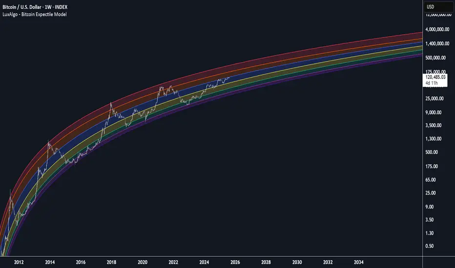
Bitcoin Expectile Model [LuxAlgo]The Bitcoin Expectile Model is a novel approach to forecasting Bitcoin, inspired by the popular Bitcoin Quantile Model by PlanC. By fitting multiple Expectile regressions to the price, we highlight zones of corrections or accumulations throughout the Bitcoin price evolution.
While we strongly recommend using this model with the Bitcoin All Time History Index INDEX:BTCUSD on the 3 days or weekly timeframe using a logarithmic scale, this model can be applied to any asset using the daily timeframe or superior.
Please note that here on TradingView, this model was solely designed to be used on the Bitcoin 1W chart, however, it can be experimented on other assets or timeframes if of interest.
🔶 USAGE
The Bitcoin Expectile Model can be applied similarly to models used for Bitcoin, highlighting lower areas of possible accumulation (support) and higher areas that allow for the anticipation of potential corrections (resistance).
By default, this model fits 7 individual Expectiles Log-Log Regressions to the price, each with their respective expectile ( tau ) values (here multiplied by 100 for the user's convenience). Higher tau values will return a fit closer to the higher highs made by the price of the asset, while lower ones will return fits closer to the lower prices observed over time.
Each zone is color-coded and has a specific interpretation. The green zone is a buy zone for long-term investing, purple is an anomaly zone for market bottoms that over-extend, while red is considered the distribution zone.
The fits can be extrapolated, helping to chart a course for the possible evolution of Bitcoin prices. Users can select the end of the forecast as a date using the "Forecast End" setting.
While the model is made for Bitcoin using a log scale, other assets showing a tendency to have a trend evolving in a single direction can be used. See the chart above on QQQ weekly using a linear scale as an example.
The Start Date can also allow fitting the model more locally, rather than over a large range of prices. This can be useful to identify potential shorter-term support/resistance areas.
🔶 DETAILS
🔹 On Quantile and Expectile Regressions
Quantile and Expectile regressions are similar; both return extremities that can be used to locate and predict prices where tops/bottoms could be more likely to occur.
The main difference lies in what we are trying to minimize, which, for Quantile regression, is commonly known as Quantile loss (or pinball loss), and for Expectile regression, simply Expectile loss.
You may refer to external material to go more in-depth about these loss functions; however, while they are similar and involve weighting specific prices more than others relative to our parameter tau, Quantile regression involves minimizing a weighted mean absolute error, while Expectile regression minimizes a weighted squared error.
The squared error here allows us to compute Expectile regression more easily compared to Quantile regression, using Iteratively reweighted least squares. For Quantile regression, a more elaborate method is needed.
In terms of comparison, Quantile regression is more robust, and easier to interpret, with quantiles being related to specific probabilities involving the underlying cumulative distribution function of the dataset; on the other expectiles are harder to interpret.
🔹 Trimming & Alterations
It is common to observe certain models ignoring very early Bitcoin price ranges. By default, we start our fit at the date 2010-07-16 to align with existing models.
By default, the model uses the number of time units (days, weeks...etc) elapsed since the beginning of history + 1 (to avoid NaN with log) as independent variable, however the Bitcoin All Time History Index INDEX:BTCUSD do not include the genesis block, as such users can correct for this by enabling the "Correct for Genesis block" setting, which will add the amount of missed bars from the Genesis block to the start oh the chart history.
🔶 SETTINGS
Start Date: Starting interval of the dataset used for the fit.
Correct for genesis block: When enabled, offset the X axis by the number of bars between the Bitcoin genesis block time and the chart starting time.
🔹 Expectiles
Toggle: Enable fit for the specified expectile. Disabling one fit will make the script faster to compute.
Expectile: Expectile (tau) value multiplied by 100 used for the fit. Higher values will produce fits that are located near price tops.
🔹 Forecast
Forecast End: Time at which the forecast stops.
🔹 Model Fit
Iterations Number: Number of iterations performed during the reweighted least squares process, with lower values leading to less accurate fits, while higher values will take more time to compute.
UM VIX status table and Roll Yield with EMA
Description :
This oscillator indicator gives you a quick snapshot of VIX, VIX futures prices, and the related VIX roll yield at a glance. When the roll yield is greater than 0, The front-month VX1 future contract is less than the next-month VX2 contract. This is called Contango and is typical for the majority of the time. If the roll yield falls below zero. This is considered backwardation where the front-month VX1 contract is higher than the value of the next-month VX2 contract. Contango is most common. When Backwardation occurs, there is usually high volatility present.
Features :
The red and green fill indicate the current roll yield with the gray line being zero.
An Exponential moving average is overlaid on the roll yield. It is red when trending down and green when trending up. If you right-click the indicator, you can set alerts for roll yield EMA color transitions green to red or red to green.
Suggested uses:
The author suggests a one hour chart using the 55 period EMA with a 60 minute setting in the indicator. This gives you a visual idea of whether the roll yield is rising or falling. The roll yield will often change directions at market turning points. For example if the roll yield EMA changes from red to green, this indicates a rising roll yield and volatility is subsiding. This could be considered bullish. If the roll yield begins falling, this indicates volatility is rising. This may be negative for stocks and indexes.
I look for short volatility positions (SVIX) when the roll yield is rising. I look for long volatility positions (VXX, UVXY, UVIX) when the roll yield begins falling. The indicator can be added to any chart. I suggest using the VX1, SPY, VIX, or other major stock index.
Set the time frame to your trading style. The default is 60 minutes. Note, the timeframe of the indicator does NOT utilize the current chart timeframe, it must be set to the desired timeframe. I manually input text on the chart indicator for understanding periods of Long and Short Volatility.
Settings and Defaults
The EMA is set to 55 by default and the table location is set to the lower right. The default time frame is 60 minutes. These features are all user configurable.
Other considerations
Sometimes the Tradingview data when a VX contract expires and another contract begins, may not transition cleanly and appear as a break on the chart. Tradingview is working on this as stated from my last request. This VX contract from one expiring contract to the next can be fixed on the price chart manually: ( Chart settings, Symbol, check the "Adjust for contract changes" box)
Observations
Pull up a one-hour chart of VX1 or SPY. Add this indicator. roll it back in time to see how the market and volatility reacts when the EMA changes from red to green and green to red. Adjust the EMA to your trading style and time frame. Use this for added confirmation of your long and short volatility trades with the Volatility ETFs SVIX, SVXY, VXX, UVXY, UVIX. or use it for long/short indexes such as SPY.

Back to zero: Understanding seriestype: pine series basic example
time required: 10 minutes
level: medium (need to know the "array" data variable as a generic programming concept, basic Pine syntax)
tl;dr how variables and series work in Pine
Pine is an array/vector language. That's something that twists how it behaves, and how we have to think about it. A lot of misunderstandings come from forgetting this fact. This example tries to clear that concept.
First, you need to know what an array is, and how it works in a programmig language. Also, having javascript under your belt helps too. If you don't, google "javascript array basic tutorial" is your friend :)
So, in pine arrays are called "series". Every variable is an array with values for each candle in the chart. if we do:
myVar = true
this is not a constant. It is a series of values for each candle, { true, true,....., true }
In practice, the result is the same, but we can access each of the values in the series, like myVar{0}, myVar{7}, myVar{anyNumber}....
Again, it is not a constant, since you can access/modify the each value individually
so, lets show it:
plot (myVar, clolor = gray)
this plots an horizontal line of value 1 ( 1 is equal to true ) so it's all good.
On to a more usual series:
tipicalSeries = close > open ? true : false
plot(tipicalSeries, color= blue)
This gives the expected result, a tipical up and down line with values at 1 or 0. Naturally, "tipicalSeries" is an array, the "ups" and "downs" are all stored under the same variable, indexed by the candles.
In Pine, the ZERO position in the array is the last one, which corresponds to the last candle on the right. Say you have a chart with 12 candles. The close would be the closing value of what we intuitively think as first candle, the one on the left. then close ... and so on.... until close , the value of the "last" candle, the one on the right. It actually helps to start thinking of the positions backwards, counting down to zero, rocket launch style :)
And back to our series. The myVar will also be the same size, from myVar to myVar .
When we do some operation with them, something simple like
if ( myVar == tipicalSeries)
what is really happening is that internally, Pine is checking each of the indexes, as in myVar == tipicalSeries , myVar == tipicalSeries .... myVar == tipicalSeries
And we can store that stuff to check it. simply:
result = (myVar == tipicalSeries) ? true : false //yes, this is the same as tipicalSeries, but we're not in a boolean logic tut ;)
plot (result)
The reason we can plot the result is that it is an array, not a single value. The example indicator i provide shows a plot where the values are obtained from different places in the array, this line here:
mySeries3 = mySeries2 and mySeries1
this creates a series that is the result of the PREVIOUS values stored (the zero index is the one most at the right, or the "current" one), which here just causes a shift in the plotted line by one candle.
Go ahead, grab a copy of my code, try to change the indexes and see the results. Understanding this stuff is critical to go deeper into Pine :)

Seasonality Monte Carlo Forecaster [BackQuant]Seasonality Monte Carlo Forecaster
Plain-English overview
This tool projects a cone of plausible future prices by combining two ideas that traders already use intuitively: seasonality and uncertainty. It watches how your market typically behaves around this calendar date, turns that seasonal tendency into a small daily “drift,” then runs many randomized price paths forward to estimate where price could land tomorrow, next week, or a month from now. The result is a probability cone with a clear expected path, plus optional overlays that show how past years tended to move from this point on the calendar. It is a planning tool, not a crystal ball: the goal is to quantify ranges and odds so you can size, place stops, set targets, and time entries with more realism.
What Monte Carlo is and why quants rely on it
• Definition . Monte Carlo simulation is a way to answer “what might happen next?” when there is randomness in the system. Instead of producing a single forecast, it generates thousands of alternate futures by repeatedly sampling random shocks and adding them to a model of how prices evolve.
• Why it is used . Markets are noisy. A single point forecast hides risk. Monte Carlo gives a distribution of outcomes so you can reason in probabilities: the median path, the 68% band, the 95% band, tail risks, and the chance of hitting a specific level within a horizon.
• Core strengths in quant finance .
– Path-dependent questions : “What is the probability we touch a stop before a target?” “What is the expected drawdown on the way to my objective?”
– Pricing and risk : Useful for path-dependent options, Value-at-Risk (VaR), expected shortfall (CVaR), stress paths, and scenario analysis when closed-form formulas are unrealistic.
– Planning under uncertainty : Portfolio construction and rebalancing rules can be tested against a cloud of plausible futures rather than a single guess.
• Why it fits trading workflows . It turns gut feel like “seasonality is supportive here” into quantitative ranges: “median path suggests +X% with a 68% band of ±Y%; stop at Z has only ~16% odds of being tagged in N days.”
How this indicator builds its probability cone
1) Seasonal pattern discovery
The script builds two day-of-year maps as new data arrives:
• A return map where each calendar day stores an exponentially smoothed average of that day’s log return (yesterday→today). The smoothing (90% old, 10% new) behaves like an EWMA, letting older seasons matter while adapting to new information.
• A volatility map that tracks the typical absolute return for the same calendar day.
It calculates the day-of-year carefully (with leap-year adjustment) and indexes into a 365-slot seasonal array so “March 18” is compared with past March 18ths. This becomes the seasonal bias that gently nudges simulations up or down on each forecast day.
2) Choice of randomness engine
You can pick how the future shocks are generated:
• Daily mode uses a Gaussian draw with the seasonal bias as the mean and a volatility that comes from realized returns, scaled down to avoid over-fitting. It relies on the Box–Muller transform internally to turn two uniform random numbers into one normal shock.
• Weekly mode uses bootstrap sampling from the seasonal return history (resampling actual historical daily drifts and then blending in a fraction of the seasonal bias). Bootstrapping is robust when the empirical distribution has asymmetry or fatter tails than a normal distribution.
Both modes seed their random draws deterministically per path and day, which makes plots reproducible bar-to-bar and avoids flickering bands.
3) Volatility scaling to current conditions
Markets do not always live in average volatility. The engine computes a simple volatility factor from ATR(20)/price and scales the simulated shocks up or down within sensible bounds (clamped between 0.5× and 2.0×). When the current regime is quiet, the cone narrows; when ranges expand, the cone widens. This prevents the classic mistake of projecting calm markets into a storm or vice versa.
4) Many futures, summarized by percentiles
The model generates a matrix of price paths (capped at 100 runs for performance inside TradingView), each path stepping forward for your selected horizon. For each forecast day it sorts the simulated prices and pulls key percentiles:
• 5th and 95th → approximate 95% band (outer cone).
• 16th and 84th → approximate 68% band (inner cone).
• 50th → the median or “expected path.”
These are drawn as polylines so you can immediately see central tendency and dispersion.
5) A historical overlay (optional)
Turn on the overlay to sketch a dotted path of what a purely seasonal projection would look like for the next ~30 days using only the return map, no randomness. This is not a forecast; it is a visual reminder of the seasonal drift you are biasing toward.
Inputs you control and how to think about them
Monte Carlo Simulation
• Price Series for Calculation . The source series, typically close.
• Enable Probability Forecasts . Master switch for simulation and drawing.
• Simulation Iterations . Requested number of paths to run. Internally capped at 100 to protect performance, which is generally enough to estimate the percentiles for a trading chart. If you need ultra-smooth bands, shorten the horizon.
• Forecast Days Ahead . The length of the cone. Longer horizons dilute seasonal signal and widen uncertainty.
• Probability Bands . Draw all bands, just 95%, just 68%, or a custom level (display logic remains 68/95 internally; the custom number is for labeling and color choice).
• Pattern Resolution . Daily leans on day-of-year effects like “turn-of-month” or holiday patterns. Weekly biases toward day-of-week tendencies and bootstraps from history.
• Volatility Scaling . On by default so the cone respects today’s range context.
Plotting & UI
• Probability Cone . Plots the outer and inner percentile envelopes.
• Expected Path . Plots the median line through the cone.
• Historical Overlay . Dotted seasonal-only projection for context.
• Band Transparency/Colors . Customize primary (outer) and secondary (inner) band colors and the mean path color. Use higher transparency for cleaner charts.
What appears on your chart
• A cone starting at the most recent bar, fanning outward. The outer lines are the ~95% band; the inner lines are the ~68% band.
• A median path (default blue) running through the center of the cone.
• An info panel on the final historical bar that summarizes simulation count, forecast days, number of seasonal patterns learned, the current day-of-year, expected percentage return to the median, and the approximate 95% half-range in percent.
• Optional historical seasonal path drawn as dotted segments for the next 30 bars.
How to use it in trading
1) Position sizing and stop logic
The cone translates “volatility plus seasonality” into distances.
• Put stops outside the inner band if you want only ~16% odds of a stop-out due to noise before your thesis can play.
• Size positions so that a test of the inner band is survivable and a test of the outer band is rare but acceptable.
• If your target sits inside the 68% band at your horizon, the payoff is likely modest; outside the 68% but inside the 95% can justify “one-good-push” trades; beyond the 95% band is a low-probability flyer—consider scaling plans or optionality.
2) Entry timing with seasonal bias
When the median path slopes up from this calendar date and the cone is relatively narrow, a pullback toward the lower inner band can be a high-quality entry with a tight invalidation. If the median slopes down, fade rallies toward the upper band or step aside if it clashes with your system.
3) Target selection
Project your time horizon to N bars ahead, then pick targets around the median or the opposite inner band depending on your style. You can also anchor dynamic take-profits to the moving median as new bars arrive.
4) Scenario planning & “what-ifs”
Before events, glance at the cone: if the 95% band already spans a huge range, trade smaller, expect whips, and avoid placing stops at obvious band edges. If the cone is unusually tight, consider breakout tactics and be ready to add if volatility expands beyond the inner band with follow-through.
5) Options and vol tactics
• When the cone is tight : Prefer long gamma structures (debit spreads) only if you expect a regime shift; otherwise premium selling may dominate.
• When the cone is wide : Debit structures benefit from range; credit spreads need wider wings or smaller size. Align with your separate IV metrics.
Reading the probability cone like a pro
• Cone slope = seasonal drift. Upward slope means the calendar has historically favored positive drift from this date, downward slope the opposite.
• Cone width = regime volatility. A widening fan tells you that uncertainty grows fast; a narrow cone says the market typically stays contained.
• Mean vs. price gap . If spot trades well above the median path and the upper band, mean-reversion risk is high. If spot presses the lower inner band in an up-sloping cone, you are in the “buy fear” zone.
• Touches and pierces . Touching the inner band is common noise; piercing it with momentum signals potential regime change; the outer band should be rare and often brings snap-backs unless there is a structural catalyst.
Methodological notes (what the code actually does)
• Log returns are used for additivity and better statistical behavior: sim_ret is applied via exp(sim_ret) to evolve price.
• Seasonal arrays are updated online with EWMA (90/10) so the model keeps learning as each bar arrives.
• Leap years are handled; indexing still normalizes into a 365-slot map so the seasonal pattern remains stable.
• Gaussian engine (Daily mode) centers shocks on the seasonal bias with a conservative standard deviation.
• Bootstrap engine (Weekly mode) resamples from observed seasonal returns and adds a fraction of the bias, which captures skew and fat tails better.
• Volatility adjustment multiplies each daily shock by a factor derived from ATR(20)/price, clamped between 0.5 and 2.0 to avoid extreme cones.
• Performance guardrails : simulations are capped at 100 paths; the probability cone uses polylines (no heavy fills) and only draws on the last confirmed bar to keep charts responsive.
• Prerequisite data : at least ~30 seasonal entries are required before the model will draw a cone; otherwise it waits for more history.
Strengths and limitations
• Strengths :
– Probabilistic thinking replaces single-point guessing.
– Seasonality adds a small but meaningful directional bias that many markets exhibit.
– Volatility scaling adapts to the current regime so the cone stays realistic.
• Limitations :
– Seasonality can break around structural changes, policy shifts, or one-off events.
– The number of paths is performance-limited; percentile estimates are good for trading, not for academic precision.
– The model assumes tomorrow’s randomness resembles recent randomness; if regime shifts violently, the cone will lag until the EWMA adapts.
– Holidays and missing sessions can thin the seasonal sample for some assets; be cautious with very short histories.
Tuning guide
• Horizon : 10–20 bars for tactical trades; 30+ for swing planning when you care more about broad ranges than precise targets.
• Iterations : The default 100 is enough for stable 5/16/50/84/95 percentiles. If you crave smoother lines, shorten the horizon or run on higher timeframes.
• Daily vs. Weekly : Daily for equities and crypto where month-end and turn-of-month effects matter; Weekly for futures and FX where day-of-week behavior is strong.
• Volatility scaling : Keep it on. Turn off only when you intentionally want a “pure seasonality” cone unaffected by current turbulence.
Workflow examples
• Swing continuation : Cone slopes up, price pulls into the lower inner band, your system fires. Enter near the band, stop just outside the outer line for the next 3–5 bars, target near the median or the opposite inner band.
• Fade extremes : Cone is flat or down, price gaps to the upper outer band on news, then stalls. Favor mean-reversion toward the median, size small if volatility scaling is elevated.
• Event play : Before CPI or earnings on a proxy index, check cone width. If the inner band is already wide, cut size or prefer options structures that benefit from range.
Good habits
• Pair the cone with your entry engine (breakout, pullback, order flow). Let Monte Carlo do range math; let your system do signal quality.
• Do not anchor blindly to the median; recalc after each bar. When the cone’s slope flips or width jumps, the plan should adapt.
• Validate seasonality for your symbol and timeframe; not every market has strong calendar effects.
Summary
The Seasonality Monte Carlo Forecaster wraps institutional risk planning into a single overlay: a data-driven seasonal drift, realistic volatility scaling, and a probabilistic cone that answers “where could we be, with what odds?” within your trading horizon. Use it to place stops where randomness is less likely to take you out, to set targets aligned with realistic travel, and to size positions with confidence born from distributions rather than hunches. It will not predict the future, but it will keep your decisions anchored to probabilities—the language markets actually speak.

PROWIN STUDY BITCOIN DOMINANCE CYCLE**Title: PROWIN STUDY BITCOIN DOMINANCE CYCLE**
**Overview:**
This TradingView script analyzes the relationship between Bitcoin dominance and Bitcoin price movements, as well as the performance of altcoins. It categorizes market conditions into different scenarios based on the movements of Bitcoin dominance and Bitcoin price, and plots the Exponential Moving Average (EMA) of the altcoins index.
**Key Components:**
1. **Bitcoin Dominance:**
- `dominanceBTC`: Fetches the Bitcoin dominance from the "CRYPTOCAP:BTC.D" symbol for the current timeframe.
2. **Bitcoin Price:**
- `priceBTC`: Uses the closing price of Bitcoin from the current chart (assumed to be BTC/USD).
3. **Altcoins Index:**
- `altcoinsIndex`: Fetches the total market cap of altcoins (excluding Bitcoin) from the "CRYPTOCAP:TOTAL2" symbol.
4. **EMA of Altcoins:**
- `emaAltcoins`: Calculates the 20-period Exponential Moving Average (EMA) of the altcoins index.
**Conditions:**
1. **Bitcoin Dominance and Price Up:**
- `dominanceBTC_up`: Bitcoin dominance crosses above its 20-period Simple Moving Average (SMA).
- `priceBTC_up`: Bitcoin price crosses above its 20-period SMA.
2. **Bitcoin Dominance Up and Price Down:**
- `priceBTC_down`: Bitcoin price crosses below its 20-period SMA.
3. **Bitcoin Dominance Up and Price Sideways:**
- `priceBTC_lateral`: Bitcoin price change is less than 5% of its 10-period average change.
4. **Altseason:**
- `altseason_condition`: Bitcoin dominance crosses below its 20-period SMA while Bitcoin price crosses above its 20-period SMA.
5. **Dump:**
- `dump_altcoins_condition`: Bitcoin dominance crosses below its 20-period SMA while Bitcoin price crosses below its 20-period SMA.
6. **Altcoins Up:**
- `altcoins_up_condition`: Bitcoin dominance crosses below its 20-period SMA while Bitcoin price moves sideways.
**Current Condition:**
- Determines the current market condition based on the above scenarios and stores it in the `currentCondition` variable.
**Plotting:**
- Plots the EMA of the altcoins index on the chart in green with a linewidth of 2.
- Displays the current market condition in a table at the top-right of the chart, with appropriate background and text colors.
**Background Color:**
- Sets a semi-transparent blue background color for the chart.
This script helps traders visualize and understand the market dynamics between Bitcoin dominance, Bitcoin price, and altcoin performance, providing insights into different market cycles and potential trading opportunities.
BTC Supply in Profits and Losses (BTCSPL) [AlgoAlpha]Description:
🚨The BTC Supply in Profits and Losses (BTCSPL) indicator, developed by AlgoAlpha, offers traders insights into the distribution of INDEX:BTCUSD addresses between profits and losses based on INDEX:BTCUSD on-chain data.
Features:
🔶Alpha Decay Adjustment: The indicator provides the option to adjust the data against Alpha Decay, this compensates for the reduction in clarity of the signal over time.
🔶Rolling Change Display: The indicator enables the display of the rolling change in the distribution of Bitcoin addresses between profits and losses, aiding in identifying shifts in market sentiment.
🔶BTCSPL Value Score: The indicator optionally displays a value score ranging from -1 to 1, traders can use this to carry out strategic dollar cost averaging and reverse dollar cost averaging based on the implied value of bitcoin.
🔶Reversal Signals: The indicator gives long-term reversal signals denoted as "▲" and "▼" for the price of bitcoin based on oversold and overbought conditions of the BTCSPL.
🔶Moving Average Visualization: Traders can choose to display a moving average line, allowing for better trend identification.
How to Use ☝️ (summary):
Alpha Decay Adjustment: Toggle this option to enable or disable Alpha Decay adjustment for a normalized representation of the data.
Moving Average: Toggle this option to show or hide the moving average line, helping traders identify trends.
Short-Term Trend: Enable this option to display the short-term trend based on the Aroon indicator.
Rolling Change: Choose this option to visualize the rolling change in the distribution between profits and losses.
BTCSPL Value Score: Activate this option to show the BTCSPL value score, ranging from -1 to 1, 1 implies that bitcoin is extremely cheap(buy) and -1 implies bitcoin is extremely expensive(sell).
Reversal Signals: Gives binary buy and sell signals for the long term

arraysLibrary "arrays"
Library contains utility functions using arrays.
delete( arr , index)
remove an item from array at specific index. Also deletes the item
Parameters:
arr: - array from which the item needs to be deleted
index: - index of item to be deleted
Returns: void
pop( arr )
remove the last item from array. Also deletes the item
Parameters:
arr: - array from which the last item needs to be removed and deleted
Returns: void
shift( arr )
remove an item from array at index 0. Also deletes the item
Parameters:
arr: - array from which the first item needs to be removed and deleted
Returns: void
unshift( arr , val, maxItems)
add an item to the beginning of an array with max items cap
Parameters:
arr: - array to which the item needs to be added at the beginning
val: - value of item which needs to be added
maxItems: - max items array can hold. After that, items are removed from the other end
Returns: resulting array
clear( arr )
remove and delete all items in an array
Parameters:
arr: - array which needs to be cleared
Returns: void
push( arr , val, maxItems)
add an item to the end of an array with max items cap
Parameters:
arr: - array to which the item needs to be added at the beginning
val: - value of item which needs to be added
maxItems: - max items array can hold. After that, items are removed from the starting index
Returns: resulting array

Coppock Curve with Pivot Points and Divergence The Coppock Curve is a long-term price momentum indicator used primarily to recognize major downturns and upturns in a stock market index. It is calculated as a 10-month weighted moving average of the sum of the 14-month rate of change and the 11-month rate of change for the index. It is also known as the "Coppock Guide."
The Coppock formula was introduced in Barron's in 1962 by Edwin Coppock.
The Coppock Curve is a technical indicator that provides long-term buy and sell signals for major stock indexes and related ETFs based on shifts in momentum.
What Does the Coppock Curve Tell You?
The Coppock Curve was originally implemented as a long-term buy and sell indicator for major indices such as the S&P 500 and the Wilshire 5000. Often, it is used with long-term time series such as a candlestick chart, but where each candle contains a month's worth of price information.
The Difference Between the Coppock Curve and Rate of Relative Strength Index (RSI)?
The relative strength index looks at how the current price compares to prior prices, though it is calculated differently than the rate of change (ROC) indicator used in the Coppock Curve calculation. Therefore, these indicators will provide different trade signals and information.
What are those circles?
-These are Divergences. Red for Regular-Bearish. Orange for Hidden-Bearish. Green for Regular-Bullish. Aqua for Hidden-Bullish.
What are those triangles?
- These are Pivots . They show when the VPT oscillator might reverse, this is important to know because many times the price action follows this move.
Please keep in mind that this indicator is a tool and not a strategy, do not blindly trade signals, do your own research first! Use this indicator in conjunction with other indicators to get multiple confirmations.

Normalized Volatility IndicatorFrom an article by Rajesh Kayakkal:
"Early bear phase signals can help you get out of the market before it turns down. This indicator tells you how.
There are many ways to identify the trend of a financial market, the most common being the 200-day exponential moving average (Ema). When price is trending down below the 200-day Ema, the market is believed to be in a bear phase. If the market is trending up above the 200-day Ema, it is considered to be in a bull phase.
Since every indicator fails at times, I wanted to find other indicators to confirm a trend. In my quest for another indicator to determine the trend for the financial markets, I found the Cboe Volatility Index (Vix) to be a good indicator of the market direction. The Vix is calculated from the weighted average of the implied volatilities of various options on the Standard & Poor’s 500 index futures.
J. Welles Wilder’s average true range can also give an indication of the financial market trends; that is, when the market is in a bull phase, the average true range narrows, and when it is in a bear phase, the average true range expands. The normalized volatility indicator (Nvi) is based on this behavior.
Normalized volatility indicator (Nvi)
Average true range (Atr) varies depending on time. But how do we determine the phase of the financial market with Atr? Perhaps some type of ratio could give us a clue. A ratio presents a relationship of a quantity with respect to another. I did some research based on a ratio of the 64-day average true range and the end-of-day value of equity indexes such as the Standard & Poor’s 500 (Spx). I selected the 64-day period since it is close to the average number of trading days in a quarter. The ratio of the 64-day average true range and closing price does discount seasonal variations in the average true range and gives a single number that can be used to compare volatility of an instrument across many decades. I call this ratio the normalized volatility indicator.
I found an interesting correlation between Nvi and cycles of major equity market indexes. The formula for the Nvi is:
Nvi = 64 - Day average true range/End-of-day price * 100
The NVI gave advanced signals before the cyclical bear phase of SPX commenced in October 2000 and was almost on the spot with the bull phase that began in 2003 and the current secular bear market cycle, which started in November 2007."
Includes options to show inverse NVI and change the ATR length and smoothing.

Hersheys CoCo World"CoCo World" helps to answer the following question... Is this stock moving alone or with other markets? No stock is an island, so it's important to see what everyone else is doing!
With limited screen real estate, I want to see as much info as possible as I'm evaluating US equities and deciding to pull the trigger to buy and sell. My "CoCo World" indicator packs a lot of info into a small space! I got the idea when looking at some Correlation Coefficient studies, hence the name "CoCo".
First I build three series to compare percent price changes...
#1 = Stock = Your chart symbol
#2 = US Index = SPY
#3 = World Index = This is an index of the top 10 world economies using the iShares country indexes. They are weighted by GDP and then the percent price change from last to current tick are summed together. For example, the US makes up 37%, China 22%, etc.
Why use iShares instead of the world markets directly, like the China SSE or Japan Nikkei? The iShares indexes are traded live at the same time as US markets. Measuring money flow in and out of these funds should naturally reflect broad sentiment about each country.
There are Green/Red bars in the indicator space under your chart, also Green/Red background colors.
Green Bar = Stock, US and World are UP, Stock up more than US, US up more than World.
Red Bar = Stock, US and World are DOWN, Stock down more than US, US down more than World.
Green Background = positive 7 period combined average direction of Symbol/US/World
Red Background = negative 7 period combined average direction of Symbol/US/World
This indicator works great all the way down to 1-minute bars... watch for green bars at the end of down-trends and red bars signalling the end of up-trends. Use caution if entering long trades while the background is red, this means the markets are against you!
Use "CoCo World" with your other favorite indicators to get a more complete picture.
Knowledge is POWER!
Good trading, and follow me for updates!
Brian Hershey

BySq - Market PsychologyThe script I provided is a Market Psychology Index indicator for TradingView, which focuses on three key psychological market phases:
FOMO (Fear of Missing Out)
Panic Selling
Reversal
This indicator uses volume, price changes, and specific time periods to gauge market sentiment. Let me break it down:
1. Input Parameters:
FOMO Period: Defines how many bars (candles) the FOMO index will consider for its calculation.
Panic Period: Defines the period to evaluate Panic Selling.
Reversal Period: Defines the period to evaluate potential price reversals.
You can adjust these periods based on your analysis preferences. The default for each period is 14.
2. FOMO Index:
The FOMO Index aims to capture the "fear of missing out" behavior in the market.
It uses volume and price change:
Volume is compared to the Simple Moving Average (SMA) of volume over the specified period.
Price change is calculated as the percentage change in price compared to the previous bar.
If both volume and price change indicate strong upward movement, the FOMO index spikes.
3. Panic Selling Index:
The Panic Selling Index captures when traders are selling out of fear, often in a rapid or irrational way.
Similar to the FOMO Index, it considers volume and price change:
It uses volume and compares it to the SMA of volume for the panic period.
Price change is negative, meaning it considers only price drops.
When there is high volume coupled with significant price drops, it signals panic selling.
4. Reversal Index:
The Reversal Index aims to detect potential trend reversals in the market.
This index also considers volume and price change:
It focuses on upward price movement and compares volume to its SMA.
If there’s strong upward price movement along with increasing volume, it signals the possibility of a price reversal.
5. Graphical Output:
Histograms are drawn on the chart for each of the three indices:
FOMO is shown in green (indicating the presence of FOMO) and red (when the index is low).
Panic Selling is shown in orange.
Reversal is shown in purple.
The Zero Line (horizontal dotted line) helps identify when any of the indices is positive or negative.
6. Labels:
Labels for each index are shown on the chart at the relevant bar when the index spikes.
FOMO is labeled "FOMO" in green when it spikes.
Panic Selling is labeled "Panic Selling" in orange when it spikes.
Reversal is labeled "Reversal" in purple when it spikes.
Additionally, period labels show above the chart, indicating the specific periods (FOMO, Panic, and Reversal periods) currently being applied. This provides clarity on what time frame each index is analyzing.
7. How to Use:
FOMO: High values may indicate that traders are buying out of fear of missing out on a rally, suggesting a potentially overheated market.
Panic Selling: High values could suggest irrational selling behavior or capitulation, potentially marking the bottom of a downtrend.
Reversal: High values signal the potential for a market reversal, where the price could change direction due to increased volume and upward movement.
8. Visual Appearance:
The indicator’s histograms change colors based on the level of market sentiment detected. The color-coded approach provides an easy-to-read visual representation of different psychological phases in the market.
The horizontal zero line allows easy differentiation between positive and negative values.
Summary:
This script combines the psychology of the market (FOMO, Panic Selling, and Reversal) into a set of indicators that help traders identify potential turning points or emotional states in the market. By focusing on volume and price change, the script attempts to give a clear picture of market sentiment and possible future movements.

Force Volume GradientThis Pine Script is a technical indicator designed for trading platforms, specifically TradingView. It plots the Force Volume Gradient (FVG) and generates buy/sell signals based on the crossover of the FVG line and a signal line.
Key Components:
Force Index: Calculates the exponential moving average (EMA) of the product of the close price and volume.
Force Volume Gradient (FVG): Calculates the EMA of the Force Index.
Signal Line: A simple moving average (SMA) of the FVG.
Buy/Sell Signals: Generated when the FVG line crosses above/below the signal line.
How it Works:
The script calculates the Force Index, which measures the amount of energy or "force" behind price movements.
The FVG is then calculated by applying an EMA to the Force Index, smoothing out the values.
The signal line is a SMA of the FVG, providing a benchmark for buy/sell signals.
When the FVG line crosses above the signal line, a buy signal is generated. Conversely, when the FVG line crosses below the signal line, a sell signal is generated.
Trading Strategy:
This script can be used as a momentum indicator to identify potential buying or selling opportunities. Traders can use the buy/sell signals as entry/exit points, or combine the FVG with other indicators to create a more comprehensive trading strategy.
Customization:
Users can adjust the input parameters, such as the length of the Force Index and signal line, to suit their individual trading preferences.

Savitzky Golay Median Filtered RSI [BackQuant]Savitzky Golay Median Filtered RSI
Introducing BackQuant's Savitzky Golay Median Filtered RSI, a cutting-edge indicator that enhances the classic Relative Strength Index (RSI) by applying both a Savitzky-Golay filter and a median filter to provide smoother and more reliable signals. This advanced approach helps reduce noise and captures true momentum trends with greater precision. Let’s break down how the indicator works, the features it offers, and how it can improve your trading strategy.
Core Concept: Relative Strength Index (RSI)
The Relative Strength Index (RSI) is a widely used momentum oscillator that measures the speed and change of price movements. It oscillates between 0 and 100, with levels above 70 typically indicating overbought conditions and levels below 30 indicating oversold conditions. However, the standard RSI can sometimes generate noisy signals, especially in volatile markets, making it challenging to identify reliable entry and exit points.
To improve upon the traditional RSI, this indicator introduces two powerful filters: the Savitzky-Golay filter and a median filter.
Savitzky-Golay Filter: Smoothing with Precision
The Savitzky-Golay filter is a digital filtering technique used to smooth data while preserving important features, such as peaks and trends. Unlike simple moving averages that can distort important price data, the Savitzky-Golay filter uses polynomial regression to fit the data, providing a more accurate and less lagging result.
In this script, the Savitzky-Golay filter is applied to the RSI values to smooth out short-term fluctuations and provide a more reliable signal. By using a window size of 5 and a polynomial degree of 2, the filter effectively reduces noise without compromising the integrity of the underlying price movements.
Median Filter: Reducing Outliers
After applying the Savitzky-Golay filter, the median filter is applied to the smoothed RSI values. The median filter is particularly effective at removing short-lived outliers, further enhancing the accuracy of the RSI by reducing the impact of sudden and temporary price spikes or drops. This combination of filters creates an ultra-smooth RSI that is better suited for detecting true market trends.
Long and Short Signals
The Savitzky Golay Median Filtered RSI generates long and short signals based on user-defined threshold levels:
Long Signals: A long signal is triggered when the filtered RSI exceeds the Long Threshold (default set at 176). This indicates that momentum is shifting upward, and it may present a good buying opportunity.
Short Signals: A short signal is generated when the filtered RSI falls below the Short Threshold (default set at 162). This suggests that momentum is weakening, potentially signaling a selling opportunity or exit from a long position.
These threshold levels can be adjusted to suit different market conditions and timeframes, allowing traders to fine-tune the sensitivity of the indicator.
Customization and Visualization Options
The Savitzky Golay Median Filtered RSI comes with several customization options, enabling traders to tailor the indicator to their specific needs:
Calculation Source: Select the price source for the RSI calculation (default is OHLC4, but it can be changed to close, open, high, or low prices).
RSI Period: Adjust the lookback period for the RSI calculation (default is 14).
Median Filter Length: Control the length of the median filter applied to the smoothed RSI, affecting how much noise is removed from the signal.
Threshold Levels: Customize the long and short thresholds to define the sensitivity for generating buy and sell signals.
UI Settings: Choose whether to display the RSI and thresholds on the chart, color the bars according to trend direction, and adjust the line width and colors used for long and short signals.
Visual Feedback: Color-Coded Signals and Thresholds
To make the signals easier to interpret, the indicator offers visual feedback by coloring the price bars and the RSI plot according to the current market trend:
Green Bars indicate long signals when momentum is bullish.
Red Bars indicate short signals when momentum is bearish.
Gray Bars indicate neutral or undecided conditions when no clear signal is present.
In addition, the Long and Short Thresholds can be plotted directly on the chart to provide a clear reference for when signals are triggered, allowing traders to visually gauge the strength of the RSI relative to its thresholds.
Alerts for Automation
For traders who prefer automated notifications, the Savitzky Golay Median Filtered RSI includes built-in alert conditions for long and short signals. You can configure these alerts to notify you when a buy or sell condition is met, ensuring you never miss a trading opportunity.
Trading Applications
This indicator is versatile and can be used in a variety of trading strategies:
Trend Following: The combination of Savitzky-Golay and median filtering makes this RSI particularly useful for identifying strong trends without being misled by short-term noise. Traders can use the long and short signals to enter trades in the direction of the prevailing trend.
Reversal Trading: By adjusting the threshold levels, traders can use this indicator to spot potential reversals. When the RSI moves from overbought to oversold levels (or vice versa), it may signal a shift in market direction.
Swing Trading: The smoothed RSI provides a clear signal for short to medium-term price movements, making it an excellent tool for swing traders looking to capitalize on momentum shifts.
Risk Management: The filtered RSI can be used as part of a broader risk management strategy, helping traders avoid false signals and stay in trades only when the momentum is strong.
Final Thoughts
The Savitzky Golay Median Filtered RSI takes the classic RSI to the next level by applying advanced smoothing techniques that reduce noise and improve signal reliability. Whether you’re a trend follower, swing trader, or reversal trader, this indicator provides a more refined approach to momentum analysis, helping you make better-informed trading decisions.
As with all indicators, it is important to backtest thoroughly and incorporate sound risk management strategies when using the Savitzky Golay Median Filtered RSI in your trading system.
Thus following all of the key points here are some sample backtests on the 1D Chart
Disclaimer: Backtests are based off past results, and are not indicative of the future.
INDEX:BTCUSD
INDEX:ETHUSD
BINANCE:SOLUSD

Futures Globex Session(s)This indicator draws a box around the Globex Session for the various Futures markets. The box height defines the highs and lows of that session, and the width defines the timeframe of that session. The boxes are outlined green if price rose during that period, and red if price fell during that period. The default Globex Session is set for the Equity Index Futures and is set in the UTC-4 time zone (Eastern Time). In the settings you can adjust the session time and time zone of your Globex Session to reflect the trading times of that market. Below are the session times for various Futures markets set in time zone UTC-4.
Equity Indexes: 18:00 - 9:30
(ES, NQ, YM, RTY)
Treasuries: 18:00 - 8:20
(ZN, ZB)
Metals: 18:00 - 8:20
(GC)
Energies: 18:00 - 9:00
(CL, NG)
Agricultures: 20:00 - 9:30
(ZS, ZW)
IBD PowerTrendThis IBD PowerTrend indicator is designed to help traders identify strong market uptrends based on the IBD Market School's Power Trend methodology. It is intended to be added to daily charts on major indexes.
Concept and Methodology
The IBD PowerTrend helps traders identify strong market uptrends. Markets generally exist in three states: uptrends, downtrends, and rangebound motion. This methodology focuses on:
Downtrends: Stay out of the market.
Rangebound markets: Often frustrating, best avoided.
Uptrends: Identify the strongest uptrends early.
This indicator uses IBD's research on historical uptrends to help traders get in and stay in during robust market phases.
How It Works
A PowerTrend starts when the following four conditions are met simultaneously on a major index:
10-Day Low Above 21-Day EMA : The market's low must be above the 21-day exponential moving average (EMA) for at least 10 consecutive days.
21-Day EMA Above 50-Day SMA : The 21-day EMA must be above the 50-day simple moving average (SMA) for at least five consecutive days.
50-Day SMA Uptrend : The 50-day SMA must be in an uptrend (one day is sufficient).
Market Closes Up : The market must close higher than the previous day's close.
A PowerTrend typically ends when the 21-day EMA crosses back below the 50-day SMA. However, there are rare cases where a PowerTrend can end early due to a circuit breaker or a follow-through day failure. In this script, a circuit breaker is defined as a break of the 50-day line and being more than 10% below recent highs (interpreted as three months).
How to Use
When the PowerTrend is active, the indicator will plot green circles, signaling a strong market uptrend. During these periods, traders might observe opportunities in growth stocks breaking out of sound bases and consider the use of margin. Conversely, during downtrends, the indicator suggests a more defensive approach.
It is recommended to use on daily timeframe.
Chart Description
Main Chart:
- EMA 21 (blue): The 21-day exponential moving average.
- SMA 50 (red): The 50-day simple moving average.
First Panel:
- IBD PowerTrend Indicator: Plots the PowerTrend status with green circles indicating an active PowerTrend.
Second Panel:
- Volume Bars

Relative Average Extrapolation [ChartPrime]Relative Average Extrapolation (ChartPrime) is a new take on session averages, like the famous vwap . This indicator leverages patterns in the market by leveraging average-at-time to get a footprint of the average market conditions for the current time. This allows for a great estimate of market conditions throughout the day allowing for predictive forecasting. If we know what the market conditions are at a given time of day we can use this information to make assumptions about future market conditions. This is what allows us to estimate an entire session with fair accuracy. This indicator works on any intra-day time frame and will not work on time frames less than a minute, or time frames that are a day or greater in length. A unique aspect of this indicator is that it allows for analysis of pre and post market sessions independently from regular hours. This results in a cleaner and more usable vwap for each individual session. One drawback of this is that the indicator utilizes an average for the length of a session. Because of this, some after hour sessions will only have a partial estimation. The average and deviation bands will work past the point where it has been extrapolated to in this instance however. On low time frames due to the limited number of data points, the indicator can appear noisy.
Generally crypto doesn't have a consistent footprint making this indicator less suitable in crypto markets. Because of this we have implemented other weighting schemes to allow for more flexibility in the number of use cases for this indicator. Besides volume weighting we have also included time, volatility, and linear (none) weighting. Using any one of these weighting schemes will transform the vwap into a wma, volatility adjusted ma, or a simple moving average. All of the style are still session period and will become longer as the session progresses.
Relative Average Extrapolation (ChartPrime) works by storing data for each time step throughout the day by utilizing a custom indexing system. It takes the a key , ie hour/minute, and transforms it into an array index to stor the current data point in its unique array. From there we can take the current time of day and advance it by one step to retrieve the data point for the next bar index. This allows us to utilize the footprint the extrapolate into the future. We use the relative rate of change for the average, the relative deviation, and relative price position to extrapolate from the current point to the end of the session. This process is fast and effective and possibly easier to use than the built in map feature.
If you have used vwap before you should be familiar with the general settings for this indicator. We have made a point to make it as intuitive for anyone who is already used to using the standard vwap. You can pick the source for the average and adjust/enable the deviation bands multipliers in the settings group. The average period is what determines the number of days to use for the average-at-time. When it is set to 0 it will use all available data. Under "Extrapolation" you will find the settings for the estimation. "Direction Sensitivity" adjusts how sensitive the indicator is to the direction of the vwap. A higher number will allow it to change directions faster, where a lower number will make it more stable throughout the session. Under the "Style" section you will find all of the color and style adjustments to customize the appearance of this indicator.
Relative Average Extrapolation (ChartPrime) is an advanced and customizable session average indicator with the ability to estimate the direction and volatility of intra-day sessions. We hope you will find this script fascinating and useful in your trading and decision making. With its unique take on session weighting and forecasting, we believe it will be a secret weapon for traders for years to come.
Enjoy
adaptive_mfi
█ Description
Money flow an indexed value-based price and volume for the specified input length (lookback period). In summary, a momentum indicator that attempt to measure the flow of money (identify buying/selling pressure) through the asset within a specified period of time. MFI will oscillate between 0 to 100, oftentimes comprehend the analysis with oversold (20) or overbought (80) level, and a divergence that spotted to signaling a further change in trend/direction. As similar to many other indicators that use length (commonly a fixed value) as an input parameter, can be optimized by applied an adaptive filter (Ehlers), to solve the measuring cycle period. In this indicator, the adaptive measure of dominant cycle as an input parameter for the lookback period/n, will be applied to the money flow index.
█ Money Flow Index
mfi = 100 - (100/(1 + money_flow_ratio))
where:
n = int(dominant_cycle)
money_flow_ratio = n positive raw_money_flow / n negative raw_money_flow
raw_money_flow = typical_price * volume
typical_price = hlc3
█ Feature
The indicator will have a specified default parameter of: hp_period = 48; source = ohlc4
Horizontal line indicates positive/negative money flow
MFI Color Scheme: Solid; Normalized
