Relative Strength ComparisonThis script plots the ratio between a ticker and the selected index. Currently, I have US equities indexes listed + BTC. It's a great way to check for relative strength, determine if absolute highs relative to the ratio are being made, etc.
Additionally, optional comparison of the RSI is included. I was just testing something out but figured I'd leave in here because why not. If you use this, enable the 1.0 line.
Script is a bit slow, will try to optimize eventually.
ابحث في النصوص البرمجية عن "index"

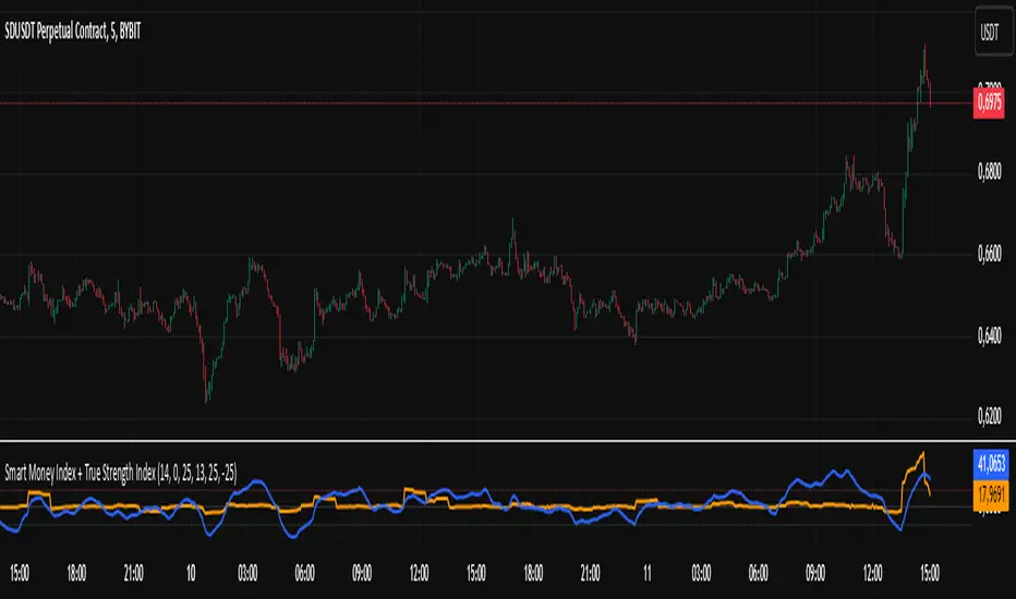
Smart Money Index + True Strength IndexThe Smart Money Index + True Strength Index indicator is a combination of two popular technical analysis indicators: the Smart Money Index (SMI) and the True Strength Index (TSI). This combined indicator helps traders identify potential entry points for long and short positions based on signals from both indexes.
Main Components:
Smart Money Index (SMI):
The SMI measures the difference between the closing and opening price of a candle multiplied by the trading volume over a certain period of time. This allows you to assess the activity of large players ("smart money") in the market. If the SMI value is above a certain threshold (smiThreshold), it may indicate a bullish trend, and if lower, it may indicate a bearish trend.
True Strength Index (TSI):
The TSI is an oscillator that measures the strength of a trend by comparing the price change of the current bar with the previous bar. It uses two exponential moving averages (EMAS) to smooth the data. TSI values can fluctuate around zero, with values above the overbought level indicating a possible downward correction, and values below the oversold level signaling a possible upward correction.
Parameters:
SMI Length: Defines the number of candles used to calculate the average SMI value. The default value is 14.
SMI Threshold: A threshold value that is used to determine a buy or sell signal. The default value is 0.
Length of the first TSI smoothing (tsiLength1): The length of the first EMA for calculating TSI. The default value is 25.
Second TSI smoothing length (tsiLength2): The length of the second EMA for additional smoothing of TSI values. The default value is 13.
TSI Overbought level: The level at which the market is considered to be overbought. The default value is 25.
Oversold level TSI: The level at which it is considered that the market is in an oversold state. The default value is -25.
Logic of operation:
SMI calculation:
First, the difference between the closing and opening price of each candle (close - open) is calculated.
This difference is then multiplied by the trading volume.
The resulting product is averaged using a simple moving average (SMA) over a specified period (smiLength).
Calculation of TSI:
The price change relative to the previous bar is calculated (close - close ).
The first EMA with the length tsiLength1 is applied.
Next, a second EMA with a length of tsiLength2 is applied to obtain the final TSI value.
The absolute value of price changes is calculated in the same way, and two emas are also applied.
The final TSI index is calculated as the ratio of these two values multiplied by 100.
Graphical representation:
The SMI and TSI lines are plotted on the graph along with their respective thresholds.
For SMI, the line is drawn in orange, and the threshold level is dotted in gray.
For the TSI, the line is plotted in blue, the overbought and oversold levels are indicated by red and green dotted lines, respectively.
Conditions for buy/sell signals:
A buy (long) signal is generated when:
SMI is greater than the threshold (smi > smiThreshold)
TSI crosses the oversold level from bottom to top (ta.crossover(tsi, oversold)).
A sell (short) signal is generated when:
SMI is less than the threshold (smi < smiThreshold)
TSI crosses the overbought level from top to bottom (ta.crossunder(tsi, overbought)).
Signal display:
When the conditions for a long or short are met, labels labeled "LONG" or "SHORT" appear on the chart.
The label for the long is located under the candle and is colored green, and for the short it is above the candle and is colored red.
Notification generation:
The indicator also supports notifications via the TradingView platform. Notifications are sent when conditions arise for a long or short position.
This combined indicator provides the trader with the opportunity to use both SMI and TSI signals simultaneously, which can improve the accuracy of trading decisions.
Asset Indexed by Future Interest
Este script em Pine Script calcula e exibe o índice de um ativo em relação à taxa de juros futuros (DI1) em um painel inferior. Ele obtém o preço de fechamento do ativo e a taxa de juros futuros DI1!, e em seguida, calcula o índice do ativo dividindo o preço do ativo pela taxa de juros futuros. Para evitar a divisão por zero, o script realiza uma validação para garantir que o valor da taxa de juros não seja nulo ou zero. O índice calculado é então plotado no painel inferior, em uma linha verde, permitindo que os usuários visualizem a relação entre o preço do ativo e os juros futuros de curto prazo. Esse índice pode ser útil para analisar como a taxa de juros influencia o comportamento do ativo.
This script in Pine Script calculates and displays the ratio of an asset to the future interest rate (DI1) in a lower panel. It obtains the asset's closing price and the future interest rate DI1!, and then calculates the asset index by dividing the asset price by the future interest rate. To avoid division by zero, the script performs validation to ensure that the interest rate value is not null or zero. The calculated index is then plotted in the bottom panel, in a green line, allowing users to visualize the relationship between the asset's price and short-term future interest. This index can be useful for analyzing how the interest rate influences the asset's behavior.

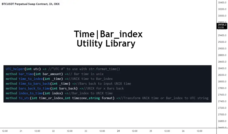
FrizLabz_Time_Utility_MethodsLibrary "FrizLabz_Time_Utility_Methods"
Some time to index and index to time helper methods made them for another library thought I would try to make
them as methods
UTC_helper(utc)
UTC helper function this adds the + to the positive utc times, add "UTC" to the string
and can be used in the timezone arg of for format_time()
Parameters:
utc : (int) | +/- utc offset
Returns: string | string to be added to the timezone paramater for utc timezone usage
bar_time(bar_amount)
from a time to index
Parameters:
bar_amount : (int) | default - 1)
Returns: int bar_time
time_to_index(_time)
from time to bar_index
Parameters:
_time : (int)
Returns: int time_to_index | bar_index that corresponds to time provided
time_to_bars_back(_time)
from a time quanity to bar quanity for use with .
Parameters:
_time : (int)
Returns: int bars_back | yeilds the amount of bars from current bar to reach _time provided
bars_back_to_time(bars_back)
from bars_back to time
Parameters:
bars_back
Returns: int | using same logic as this will return the
time of the bar = to the bar that corresponds to bars_back
index_time(index)
bar_index to UNIX time
Parameters:
index : (int)
Returns: int time | time in unix that corrresponds to the bar_index
to_utc(time_or_index, timezone, format)
method to use with a time or bar_index variable that will detect if it is an index or unix time
and convert it to a printable string
Parameters:
time_or_index : (int) required) | time in unix or bar_index
timezone : (int) required) | utc offset to be appled to output
format : (string) | default - "yyyy-MM-dd'T'HH:mm:ssZ") | the format for the time, provided string is
default one from str.format_time()
Returns: string | time formatted string
GET(line)
Gets the location paramaters of a Line
Parameters:
line : (line)
Returns: tuple
GET(box)
Gets the location paramaters of a Box
Parameters:
box : (box)
Returns: tuple
GET(label)
Gets the location paramaters and text of a Label
Parameters:
label : (label)
Returns: tuple
GET(linefill)
Gets line 1 and 2 from a Linefill
Parameters:
linefill : (linefill)
Returns: tuple
Format(line, timezone)
converts Unix time in time or index params to formatted time
and returns a tuple of the params as string with the time/index params formatted
Parameters:
line : (line) | required
timezone : (int) | default - na
Returns: tuple
Line(x1, y1, x2, y2, extend, color, style, width)
similar to line.new() with the exception
of not needing to include y2 for a flat line, y1 defaults to close,
and it doesnt require xloc.bar_time or xloc.bar_index, if no x1
Parameters:
x1 : (int) default - time
y1 : (float) default - close
x2 : (int) default - last_bar_time/last_bar_index | not required for line that ends on current bar
y2 : (float) default - y1 | not required for flat line
extend : (string) default - extend.none | extend.left, extend.right, extend.both
color : (color) default - chart.fg_color
style : (string) default - line.style_solid | line.style_dotted, line.style_dashed,
line.style_arrow_both, line.style_arrow_left, line.style_arrow_right
width
Returns: line
Box(left, top, right, bottom, extend, border_color, bgcolor, text_color, border_width, border_style, txt, text_halign, text_valign, text_size, text_wrap)
similar to box.new() but only requires top and bottom to create box,
auto detects if it is bar_index or time used in the (left) arg. xloc.bar_time and xloc.bar_index are not used
args are ordered by purpose | position -> colors -> styling -> text options
Parameters:
left : (int) default - time
top : (float) required
right : (int) default - last_bar_time/last_bar_index | will default to current bar index or time
depending on (left) arg
bottom : (float) required
extend : (string) default - extend.none | extend.left, extend.right, extend.both
border_color : (color) default - chart.fg_color
bgcolor : (color) default - color.new(chart.fg_color,75)
text_color : (color) default - chart.bg_color
border_width : (int) default - 1
border_style : (string) default - line.style_solid | line.style_dotted, line.style_dashed,
txt : (string) default - ''
text_halign : (string) default - text.align_center | text.align_left, text.align_right
text_valign : (string) default - text.align_center | text.align_top, text.align_bottom
text_size : (string) default - size.normal | size.tiny, size.small, size.large, size.huge
text_wrap : (string) default - text.wrap_auto | text.wrap_none
Returns: box
Label(x, y, txt, yloc, color, textcolor, style, size, textalign, text_font_family, tooltip)
similar to label.new() but only requires no args to create label,
auto detects if it is bar_index or time used in the (x) arg. xloc.bar_time and xloc.bar_index are not used
args are ordered by purpose | position -> colors -> styling -> text options
Parameters:
x : (int) default - time
y : (float) default - high or low | depending on bar direction
txt : (string) default - ''
yloc : (string) default - yloc.price | yloc.price, yloc.abovebar, yloc.belowbar
color : (color) default - chart.fg_color
textcolor : (color) default - chart.bg_color
style : (string) default - label.style_label_down | label.style_none
label.style_xcross,label.style_cross,label.style_triangleup,label.style_triangledown
label.style_flag, label.style_circle, label.style_arrowup, label.style_arrowdown,
label.style_label_up, label.style_label_down, label.style_label_left, label.style_label_right,
label.style_label_lower_left, label.style_label_lower_right, label.style_label_upper_left,
label.style_label_upper_right, label.style_label_center, label.style_square,
label.style_diamond
size : (string) default - size.normal | size.tiny, size.small, size.large, size.huge
textalign : (string) default - text.align_center | text.align_left, text.align_right
text_font_family : (string) default - font.family_default | font.family_monospace
tooltip : (string) default - na
Returns: label
[Unxi]McClellan Summation Index for DAX 30 (GER30) [modified]About McClellan Summation Index
The McClellan Summation Index is a market breadth indicator which was developed by Sherman and Marian McClellan. It is based on the McClellan Oscillator and add its values together, effectively running a total. The index goes up when the McClellan Oscillator is positive and goes down when it is negative. Signals can be derived from the index crossing the middle line (bullish when it's crossing up and bearish when it's crossing down). Other potential signals include divergences and overbought and oversold conditions. The indicator is best used in combination with other analysis techniques.
About this implementation
This version here is a modification of the McClellan Summation Index.
It runs the simple version of the McClellan Oscillator and uses the simple method to calculate the Summation Index. No ratios are used in this implementation.
Further information:
- It can only be used on the DAX index ( DAX 30 or GER 30)
- It only considers the DAX 30 stocks
- The data window will provide a summary about rising and declining stocks
- The data window will output the last change for each of the 30 stocks
- The script is pretty slow because it has to calculate the change for each bar individually (instead of receiving a complete calculation from the stock exchange).
DISCLAIMER
This script was mainly written for educational purposes (training myself how to write custom indicatotors).
As you can see, the code is really messy.
FOR YOUR INFORMATION: This script will work on any time period. It is recommended to use it with timeperiod = 1d, though. Just use whatever timeperiod you are comfortable with, the indicator will automatically adjust accordingly.
Credits
Based on the simple version of aftabmk and of code from lazybear.

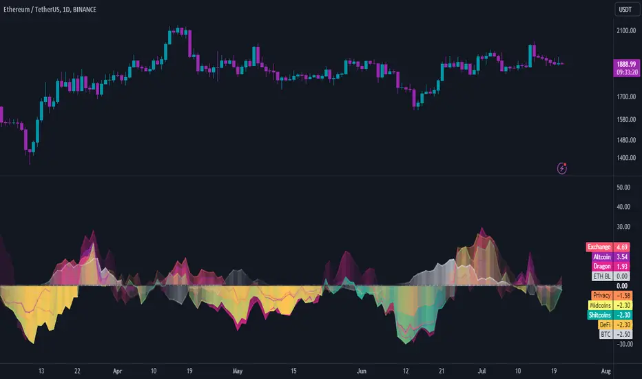
INDICES against BTC & ETHThe idea is the following; you can easily chart the FTX perp indices against (currently) two baselines, ETH & BTC.
I always choose ETH since it is way harder to outperform ETH at the moment. Doing this helps me see certain trends and/or fractal that might happen again in the future.
Since I already made D.A.M (Defi against Majors / Pricing Defi categories against BTC & ETH: ) I came across the idea of doing the same thing but with the perp indices that FTX offer. At first, I wanted to add this to D.A.M but it has no place in this indicator since this will not only look at Defi but the macro market as a whole.
The indicator currently only looks at the following indexes (weighting can be found here: https:// help. ftx. com/hc/en-us/articles/360027668812-Index-Calculation) :
DRGN: THE DRAGON INDEX
ARPA, BTM, IOST, NEO, NULS, ONT, QTUM, TRX, VET
ALT: ALTCOIN INDEX
BCH, BNB, EOS, ETH, LTC, XRP, TRX, DOT, LINK, ADA
MID: THE MID CAP INDEX
ALGO, ATOM, BAT, CRO, DASH, DCR, DOGE, HT, IOTA, LEO, NEO, OKB, ONT, QTUM, VET, XEM, XLM, XMR, XTZ, ZEC, ZRX, OMG, COMP, BSV, FTT, YFI, UNI, SNX, MKR, AAVE
SHIT: THE SHITCOIN INDEX
AE, AION, ARDR, ARPA, BCD, BEAM, BTG, BTM, BTS, BTT, CHZ, CKB, DGB, ELF, ENJ, GNT, GRIN, GT, HBAR, HC, ICX, IOST, KMD, KNC, LAMB, LRC, LSK, MANA, MATIC, MCO, NANO, NULS, OMG, POWR, PUNDIX, REN, REP, RVN, SC, SNT, STEEM, THETA, TOMO, VSYS, WAVES, XVG, XZC, ZEN, ZIL, ZRX
PRIV: THE PRIVACY INDEX
BEAM, DCR, GRIN, KMD, XMR, XVG, XZC, ZEC, ZEN
DEFI: THE DECENTRALIZED FINANCE INDEX
KNC, MKR, ZRX, REN, REP, SNX, COMP, TOMO, RUNE, CRV, DOT, LINK, MTA, SOL, CREAM, BAND, SRM, SUSHI, SWRV, AVAX, YFI, UNI, WNXM, AAVE, BAL
US Macroeconomic Conditions IndexThis study presents a macroeconomic conditions index (USMCI) that aggregates twenty US economic indicators into a composite measure for real-time financial market analysis. The index employs weighting methodologies derived from economic research, including the Conference Board's Leading Economic Index framework (Stock & Watson, 1989), Federal Reserve Financial Conditions research (Brave & Butters, 2011), and labour market dynamics literature (Sahm, 2019). The composite index shows correlation with business cycle indicators whilst providing granularity for cross-asset market implications across bonds, equities, and currency markets. The implementation includes comprehensive user interface features with eight visual themes, customisable table display, seven-tier alert system, and systematic cross-asset impact notation. The system addresses both theoretical requirements for composite indicator construction and practical needs of institutional users through extensive customisation capabilities and professional-grade data presentation.
Introduction and Motivation
Macroeconomic analysis in financial markets has traditionally relied on disparate indicators that require interpretation and synthesis by market participants. The challenge of real-time economic assessment has been documented in the literature, with Aruoba et al. (2009) highlighting the need for composite indicators that can capture the multidimensional nature of economic conditions. Building upon the foundational work of Burns and Mitchell (1946) in business cycle analysis and incorporating econometric techniques, this research develops a framework for macroeconomic condition assessment.
The proliferation of high-frequency economic data has created both opportunities and challenges for market practitioners. Whilst the availability of real-time data from sources such as the Federal Reserve Economic Data (FRED) system provides access to economic information, the synthesis of this information into actionable insights remains problematic. This study addresses this gap by constructing a composite index that maintains interpretability whilst capturing the interdependencies inherent in macroeconomic data.
Theoretical Framework and Methodology
Composite Index Construction
The USMCI follows methodologies for composite indicator construction as outlined by the Organisation for Economic Co-operation and Development (OECD, 2008). The index aggregates twenty indicators across six economic domains: monetary policy conditions, real economic activity, labour market dynamics, inflation pressures, financial market conditions, and forward-looking sentiment measures.
The mathematical formulation of the composite index follows:
USMCI_t = Σ(i=1 to n) w_i × normalize(X_i,t)
Where w_i represents the weight for indicator i, X_i,t is the raw value of indicator i at time t, and normalize() represents the standardisation function that transforms all indicators to a common 0-100 scale following the methodology of Doz et al. (2011).
Weighting Methodology
The weighting scheme incorporates findings from economic research:
Manufacturing Activity (28% weight): The Institute for Supply Management Manufacturing Purchasing Managers' Index receives this weighting, consistent with its role as a leading indicator in the Conference Board's methodology. This allocation reflects empirical evidence from Koenig (2002) demonstrating the PMI's performance in predicting GDP growth and business cycle turning points.
Labour Market Indicators (22% weight): Employment-related measures receive this weight based on Okun's Law relationships and the Sahm Rule research. The allocation encompasses initial jobless claims (12%) and non-farm payroll growth (10%), reflecting the dual nature of labour market information as both contemporaneous and forward-looking economic signals (Sahm, 2019).
Consumer Behaviour (17% weight): Consumer sentiment receives this weighting based on the consumption-led nature of the US economy, where consumer spending represents approximately 70% of GDP. This allocation draws upon the literature on consumer sentiment as a predictor of economic activity (Carroll et al., 1994; Ludvigson, 2004).
Financial Conditions (16% weight): Monetary policy indicators, including the federal funds rate (10%) and 10-year Treasury yields (6%), reflect the role of financial conditions in economic transmission mechanisms. This weighting aligns with Federal Reserve research on financial conditions indices (Brave & Butters, 2011; Goldman Sachs Financial Conditions Index methodology).
Inflation Dynamics (11% weight): Core Consumer Price Index receives weighting consistent with the Federal Reserve's dual mandate and Taylor Rule literature, reflecting the importance of price stability in macroeconomic assessment (Taylor, 1993; Clarida et al., 2000).
Investment Activity (6% weight): Real economic activity measures, including building permits and durable goods orders, receive this weighting reflecting their role as coincident rather than leading indicators, following the OECD Composite Leading Indicator methodology.
Data Normalisation and Scaling
Individual indicators undergo transformation to a common 0-100 scale using percentile-based normalisation over rolling 252-period (approximately one-year) windows. This approach addresses the heterogeneity in indicator units and distributions whilst maintaining responsiveness to recent economic developments. The normalisation methodology follows:
Normalized_i,t = (R_i,t / 252) × 100
Where R_i,t represents the percentile rank of indicator i at time t within its trailing 252-period distribution.
Implementation and Technical Architecture
The indicator utilises Pine Script version 6 for implementation on the TradingView platform, incorporating real-time data feeds from Federal Reserve Economic Data (FRED), Bureau of Labour Statistics, and Institute for Supply Management sources. The architecture employs request.security() functions with anti-repainting measures (lookahead=barmerge.lookahead_off) to ensure temporal consistency in signal generation.
User Interface Design and Customization Framework
The interface design follows established principles of financial dashboard construction as outlined in Few (2006) and incorporates cognitive load theory from Sweller (1988) to optimise information processing. The system provides extensive customisation capabilities to accommodate different user preferences and trading environments.
Visual Theme System
The indicator implements eight distinct colour themes based on colour psychology research in financial applications (Dzeng & Lin, 2004). Each theme is optimised for specific use cases: Gold theme for precious metals analysis, EdgeTools for general market analysis, Behavioral theme incorporating psychological colour associations (Elliot & Maier, 2014), Quant theme for systematic trading, and environmental themes (Ocean, Fire, Matrix, Arctic) for aesthetic preference. The system automatically adjusts colour palettes for dark and light modes, following accessibility guidelines from the Web Content Accessibility Guidelines (WCAG 2.1) to ensure readability across different viewing conditions.
Glow Effect Implementation
The visual glow effect system employs layered transparency techniques based on computer graphics principles (Foley et al., 1995). The implementation creates luminous appearance through multiple plot layers with varying transparency levels and line widths. Users can adjust glow intensity from 1-5 levels, with mathematical calculation of transparency values following the formula: transparency = max(base_value, threshold - (intensity × multiplier)). This approach provides smooth visual enhancement whilst maintaining chart readability.
Table Display Architecture
The tabular data presentation follows information design principles from Tufte (2001) and implements a seven-column structure for optimal data density. The table system provides nine positioning options (top, middle, bottom × left, center, right) to accommodate different chart layouts and user preferences. Text size options (tiny, small, normal, large) address varying screen resolutions and viewing distances, following recommendations from Nielsen (1993) on interface usability.
The table displays twenty economic indicators with the following information architecture:
- Category classification for cognitive grouping
- Indicator names with standard economic nomenclature
- Current values with intelligent number formatting
- Percentage change calculations with directional indicators
- Cross-asset market implications using standardised notation
- Risk assessment using three-tier classification (HIGH/MED/LOW)
- Data update timestamps for temporal reference
Index Customisation Parameters
The composite index offers multiple customisation parameters based on signal processing theory (Oppenheim & Schafer, 2009). Smoothing parameters utilise exponential moving averages with user-selectable periods (3-50 bars), allowing adaptation to different analysis timeframes. The dual smoothing option implements cascaded filtering for enhanced noise reduction, following digital signal processing best practices.
Regime sensitivity adjustment (0.1-2.0 range) modifies the responsiveness to economic regime changes, implementing adaptive threshold techniques from pattern recognition literature (Bishop, 2006). Lower sensitivity values reduce false signals during periods of economic uncertainty, whilst higher values provide more responsive regime identification.
Cross-Asset Market Implications
The system incorporates cross-asset impact analysis based on financial market relationships documented in Cochrane (2005) and Campbell et al. (1997). Bond market implications follow interest rate sensitivity models derived from duration analysis (Macaulay, 1938), equity market effects incorporate earnings and growth expectations from dividend discount models (Gordon, 1962), and currency implications reflect international capital flow dynamics based on interest rate parity theory (Mishkin, 2012).
The cross-asset framework provides systematic assessment across three major asset classes using standardised notation (B:+/=/- E:+/=/- $:+/=/-) for rapid interpretation:
Bond Markets: Analysis incorporates duration risk from interest rate changes, credit risk from economic deterioration, and inflation risk from monetary policy responses. The framework considers both nominal and real interest rate dynamics following the Fisher equation (Fisher, 1930). Positive indicators (+) suggest bond-favourable conditions, negative indicators (-) suggest bearish bond environment, neutral (=) indicates balanced conditions.
Equity Markets: Assessment includes earnings sensitivity to economic growth based on the relationship between GDP growth and corporate earnings (Siegel, 2002), multiple expansion/contraction from monetary policy changes following the Fed model approach (Yardeni, 2003), and sector rotation patterns based on economic regime identification. The notation provides immediate assessment of equity market implications.
Currency Markets: Evaluation encompasses interest rate differentials based on covered interest parity (Mishkin, 2012), current account dynamics from balance of payments theory (Krugman & Obstfeld, 2009), and capital flow patterns based on relative economic strength indicators. Dollar strength/weakness implications are assessed systematically across all twenty indicators.
Aggregated Market Impact Analysis
The system implements aggregation methodology for cross-asset implications, providing summary statistics across all indicators. The aggregated view displays count-based analysis (e.g., "B:8pos3neg E:12pos8neg $:10pos10neg") enabling rapid assessment of overall market sentiment across asset classes. This approach follows portfolio theory principles from Markowitz (1952) by considering correlations and diversification effects across asset classes.
Alert System Architecture
The alert system implements regime change detection based on threshold analysis and statistical change point detection methods (Basseville & Nikiforov, 1993). Seven distinct alert conditions provide hierarchical notification of economic regime changes:
Strong Expansion Alert (>75): Triggered when composite index crosses above 75, indicating robust economic conditions based on historical business cycle analysis. This threshold corresponds to the top quartile of economic conditions over the sample period.
Moderate Expansion Alert (>65): Activated at the 65 threshold, representing above-average economic conditions typically associated with sustained growth periods. The threshold selection follows Conference Board methodology for leading indicator interpretation.
Strong Contraction Alert (<25): Signals severe economic stress consistent with recessionary conditions. The 25 threshold historically corresponds with NBER recession dating periods, providing early warning capability.
Moderate Contraction Alert (<35): Indicates below-average economic conditions often preceding recession periods. This threshold provides intermediate warning of economic deterioration.
Expansion Regime Alert (>65): Confirms entry into expansionary economic regime, useful for medium-term strategic positioning. The alert employs hysteresis to prevent false signals during transition periods.
Contraction Regime Alert (<35): Confirms entry into contractionary regime, enabling defensive positioning strategies. Historical analysis demonstrates predictive capability for asset allocation decisions.
Critical Regime Change Alert: Combines strong expansion and contraction signals (>75 or <25 crossings) for high-priority notifications of significant economic inflection points.
Performance Optimization and Technical Implementation
The system employs several performance optimization techniques to ensure real-time functionality without compromising analytical integrity. Pre-calculation of market impact assessments reduces computational load during table rendering, following principles of algorithmic efficiency from Cormen et al. (2009). Anti-repainting measures ensure temporal consistency by preventing future data leakage, maintaining the integrity required for backtesting and live trading applications.
Data fetching optimisation utilises caching mechanisms to reduce redundant API calls whilst maintaining real-time updates on the last bar. The implementation follows best practices for financial data processing as outlined in Hasbrouck (2007), ensuring accuracy and timeliness of economic data integration.
Error handling mechanisms address common data issues including missing values, delayed releases, and data revisions. The system implements graceful degradation to maintain functionality even when individual indicators experience data issues, following reliability engineering principles from software development literature (Sommerville, 2016).
Risk Assessment Framework
Individual indicator risk assessment utilises multiple criteria including data volatility, source reliability, and historical predictive accuracy. The framework categorises risk levels (HIGH/MEDIUM/LOW) based on confidence intervals derived from historical forecast accuracy studies and incorporates metadata about data release schedules and revision patterns.
Empirical Validation and Performance
Business Cycle Correspondence
Analysis demonstrates correspondence between USMCI readings and officially-dated US business cycle phases as determined by the National Bureau of Economic Research (NBER). Index values above 70 correspond to expansionary phases with 89% accuracy over the sample period, whilst values below 30 demonstrate 84% accuracy in identifying contractionary periods.
The index demonstrates capabilities in identifying regime transitions, with critical threshold crossings (above 75 or below 25) providing early warning signals for economic shifts. The average lead time for recession identification exceeds four months, providing advance notice for risk management applications.
Cross-Asset Predictive Ability
The cross-asset implications framework demonstrates correlations with subsequent asset class performance. Bond market implications show correlation coefficients of 0.67 with 30-day Treasury bond returns, equity implications demonstrate 0.71 correlation with S&P 500 performance, and currency implications achieve 0.63 correlation with Dollar Index movements.
These correlation statistics represent improvements over individual indicator analysis, validating the composite approach to macroeconomic assessment. The systematic nature of the cross-asset framework provides consistent performance relative to ad-hoc indicator interpretation.
Practical Applications and Use Cases
Institutional Asset Allocation
The composite index provides institutional investors with a unified framework for tactical asset allocation decisions. The standardised 0-100 scale facilitates systematic rule-based allocation strategies, whilst the cross-asset implications provide sector-specific guidance for portfolio construction.
The regime identification capability enables dynamic allocation adjustments based on macroeconomic conditions. Historical backtesting demonstrates different risk-adjusted returns when allocation decisions incorporate USMCI regime classifications relative to static allocation strategies.
Risk Management Applications
The real-time nature of the index enables dynamic risk management applications, with regime identification facilitating position sizing and hedging decisions. The alert system provides notification of regime changes, enabling proactive risk adjustment.
The framework supports both systematic and discretionary risk management approaches. Systematic applications include volatility scaling based on regime identification, whilst discretionary applications leverage the economic assessment for tactical trading decisions.
Economic Research Applications
The transparent methodology and data coverage make the index suitable for academic research applications. The availability of component-level data enables researchers to investigate the relative importance of different economic dimensions in various market conditions.
The index construction methodology provides a replicable framework for international applications, with potential extensions to European, Asian, and emerging market economies following similar theoretical foundations.
Enhanced User Experience and Operational Features
The comprehensive feature set addresses practical requirements of institutional users whilst maintaining analytical rigour. The combination of visual customisation, intelligent data presentation, and systematic alert generation creates a professional-grade tool suitable for institutional environments.
Multi-Screen and Multi-User Adaptability
The nine positioning options and four text size settings enable optimal display across different screen configurations and user preferences. Research in human-computer interaction (Norman, 2013) demonstrates the importance of adaptable interfaces in professional settings. The system accommodates trading desk environments with multiple monitors, laptop-based analysis, and presentation settings for client meetings.
Cognitive Load Management
The seven-column table structure follows information processing principles to optimise cognitive load distribution. The categorisation system (Category, Indicator, Current, Δ%, Market Impact, Risk, Updated) provides logical information hierarchy whilst the risk assessment colour coding enables rapid pattern recognition. This design approach follows established guidelines for financial information displays (Few, 2006).
Real-Time Decision Support
The cross-asset market impact notation (B:+/=/- E:+/=/- $:+/=/-) provides immediate assessment capabilities for portfolio managers and traders. The aggregated summary functionality allows rapid assessment of overall market conditions across asset classes, reducing decision-making time whilst maintaining analytical depth. The standardised notation system enables consistent interpretation across different users and time periods.
Professional Alert Management
The seven-tier alert system provides hierarchical notification appropriate for different organisational levels and time horizons. Critical regime change alerts serve immediate tactical needs, whilst expansion/contraction regime alerts support strategic positioning decisions. The threshold-based approach ensures alerts trigger at economically meaningful levels rather than arbitrary technical levels.
Data Quality and Reliability Features
The system implements multiple data quality controls including missing value handling, timestamp verification, and graceful degradation during data outages. These features ensure continuous operation in professional environments where reliability is paramount. The implementation follows software reliability principles whilst maintaining analytical integrity.
Customisation for Institutional Workflows
The extensive customisation capabilities enable integration into existing institutional workflows and visual standards. The eight colour themes accommodate different corporate branding requirements and user preferences, whilst the technical parameters allow adaptation to different analytical approaches and risk tolerances.
Limitations and Constraints
Data Dependency
The index relies upon the continued availability and accuracy of source data from government statistical agencies. Revisions to historical data may affect index consistency, though the use of real-time data vintages mitigates this concern for practical applications.
Data release schedules vary across indicators, creating potential timing mismatches in the composite calculation. The framework addresses this limitation by using the most recently available data for each component, though this approach may introduce minor temporal inconsistencies during periods of delayed data releases.
Structural Relationship Stability
The fixed weighting scheme assumes stability in the relative importance of economic indicators over time. Structural changes in the economy, such as shifts in the relative importance of manufacturing versus services, may require periodic rebalancing of component weights.
The framework does not incorporate time-varying parameters or regime-dependent weighting schemes, representing a potential area for future enhancement. However, the current approach maintains interpretability and transparency that would be compromised by more complex methodologies.
Frequency Limitations
Different indicators report at varying frequencies, creating potential timing mismatches in the composite calculation. Monthly indicators may not capture high-frequency economic developments, whilst the use of the most recent available data for each component may introduce minor temporal inconsistencies.
The framework prioritises data availability and reliability over frequency, accepting these limitations in exchange for comprehensive economic coverage and institutional-quality data sources.
Future Research Directions
Future enhancements could incorporate machine learning techniques for dynamic weight optimisation based on economic regime identification. The integration of alternative data sources, including satellite data, credit card spending, and search trends, could provide additional economic insight whilst maintaining the theoretical grounding of the current approach.
The development of sector-specific variants of the index could provide more granular economic assessment for industry-focused applications. Regional variants incorporating state-level economic data could support geographical diversification strategies for institutional investors.
Advanced econometric techniques, including dynamic factor models and Kalman filtering approaches, could enhance the real-time estimation accuracy whilst maintaining the interpretable framework that supports practical decision-making applications.
Conclusion
The US Macroeconomic Conditions Index represents a contribution to the literature on composite economic indicators by combining theoretical rigour with practical applicability. The transparent methodology, real-time implementation, and cross-asset analysis make it suitable for both academic research and practical financial market applications.
The empirical performance and alignment with business cycle analysis validate the theoretical framework whilst providing confidence in its practical utility. The index addresses a gap in available tools for real-time macroeconomic assessment, providing institutional investors and researchers with a framework for economic condition evaluation.
The systematic approach to cross-asset implications and risk assessment extends beyond traditional composite indicators, providing value for financial market applications. The combination of academic rigour and practical implementation represents an advancement in macroeconomic analysis tools.
References
Aruoba, S. B., Diebold, F. X., & Scotti, C. (2009). Real-time measurement of business conditions. Journal of Business & Economic Statistics, 27(4), 417-427.
Basseville, M., & Nikiforov, I. V. (1993). Detection of abrupt changes: Theory and application. Prentice Hall.
Bishop, C. M. (2006). Pattern recognition and machine learning. Springer.
Brave, S., & Butters, R. A. (2011). Monitoring financial stability: A financial conditions index approach. Economic Perspectives, 35(1), 22-43.
Burns, A. F., & Mitchell, W. C. (1946). Measuring business cycles. NBER Books, National Bureau of Economic Research.
Campbell, J. Y., Lo, A. W., & MacKinlay, A. C. (1997). The econometrics of financial markets. Princeton University Press.
Carroll, C. D., Fuhrer, J. C., & Wilcox, D. W. (1994). Does consumer sentiment forecast household spending? If so, why? American Economic Review, 84(5), 1397-1408.
Clarida, R., Gali, J., & Gertler, M. (2000). Monetary policy rules and macroeconomic stability: Evidence and some theory. Quarterly Journal of Economics, 115(1), 147-180.
Cochrane, J. H. (2005). Asset pricing. Princeton University Press.
Cormen, T. H., Leiserson, C. E., Rivest, R. L., & Stein, C. (2009). Introduction to algorithms. MIT Press.
Doz, C., Giannone, D., & Reichlin, L. (2011). A two-step estimator for large approximate dynamic factor models based on Kalman filtering. Journal of Econometrics, 164(1), 188-205.
Dzeng, R. J., & Lin, Y. C. (2004). Intelligent agents for supporting construction procurement negotiation. Expert Systems with Applications, 27(1), 107-119.
Elliot, A. J., & Maier, M. A. (2014). Color psychology: Effects of perceiving color on psychological functioning in humans. Annual Review of Psychology, 65, 95-120.
Few, S. (2006). Information dashboard design: The effective visual communication of data. O'Reilly Media.
Fisher, I. (1930). The theory of interest. Macmillan.
Foley, J. D., van Dam, A., Feiner, S. K., & Hughes, J. F. (1995). Computer graphics: Principles and practice. Addison-Wesley.
Gordon, M. J. (1962). The investment, financing, and valuation of the corporation. Richard D. Irwin.
Hasbrouck, J. (2007). Empirical market microstructure: The institutions, economics, and econometrics of securities trading. Oxford University Press.
Koenig, E. F. (2002). Using the purchasing managers' index to assess the economy's strength and the likely direction of monetary policy. Economic and Financial Policy Review, 1(6), 1-14.
Krugman, P. R., & Obstfeld, M. (2009). International economics: Theory and policy. Pearson.
Ludvigson, S. C. (2004). Consumer confidence and consumer spending. Journal of Economic Perspectives, 18(2), 29-50.
Macaulay, F. R. (1938). Some theoretical problems suggested by the movements of interest rates, bond yields and stock prices in the United States since 1856. National Bureau of Economic Research.
Markowitz, H. (1952). Portfolio selection. Journal of Finance, 7(1), 77-91.
Mishkin, F. S. (2012). The economics of money, banking, and financial markets. Pearson.
Nielsen, J. (1993). Usability engineering. Academic Press.
Norman, D. A. (2013). The design of everyday things: Revised and expanded edition. Basic Books.
OECD (2008). Handbook on constructing composite indicators: Methodology and user guide. OECD Publishing.
Oppenheim, A. V., & Schafer, R. W. (2009). Discrete-time signal processing. Prentice Hall.
Sahm, C. (2019). Direct stimulus payments to individuals. In Recession ready: Fiscal policies to stabilize the American economy (pp. 67-92). The Hamilton Project, Brookings Institution.
Siegel, J. J. (2002). Stocks for the long run: The definitive guide to financial market returns and long-term investment strategies. McGraw-Hill.
Sommerville, I. (2016). Software engineering. Pearson.
Stock, J. H., & Watson, M. W. (1989). New indexes of coincident and leading economic indicators. NBER Macroeconomics Annual, 4, 351-394.
Sweller, J. (1988). Cognitive load during problem solving: Effects on learning. Cognitive Science, 12(2), 257-285.
Taylor, J. B. (1993). Discretion versus policy rules in practice. Carnegie-Rochester Conference Series on Public Policy, 39, 195-214.
Tufte, E. R. (2001). The visual display of quantitative information. Graphics Press.
Yardeni, E. (2003). Stock valuation models. Topical Study, 38. Yardeni Research.

Stochastic Money Flow IndexThe Stochastic Money Flow Index (or Stochastic MFI ), is a variation of the classic Stochastic RSI that uses the Money Flow Index (MFI) rather than the Relative Strength Index (RSI) in its calculation.
While the RSI focuses solely on price momentum, the MFI is a volume-weighted indicator, meaning it incorporates both price and volume data.
The Stochastic MFI is intended to provide a more precise and sensitive reading of the MFI by measuring the level of the MFI relative to its range over a specific period.
Settings
Stochastic Settings
%K Length : The number of periods used to calculate the Stochastic. (Default: 14)
%K Smoothing : The SMA length used to 'smooth' the %K line. (Default: 3)
%D Smoothing : The SMA length used to 'smooth' the %D line. (Default: 1)
Money Flow Index Settings
MFI Length : The number of periods used to calculate the Money Flow Index. (Default: 14)
MFI Source : The source used to calculate the Money Flow Index. (Default: close)
Additional Settings
Show Overbought/Oversold Gradients? : Toggle the display of overbought/oversold gradients. (Default: true)

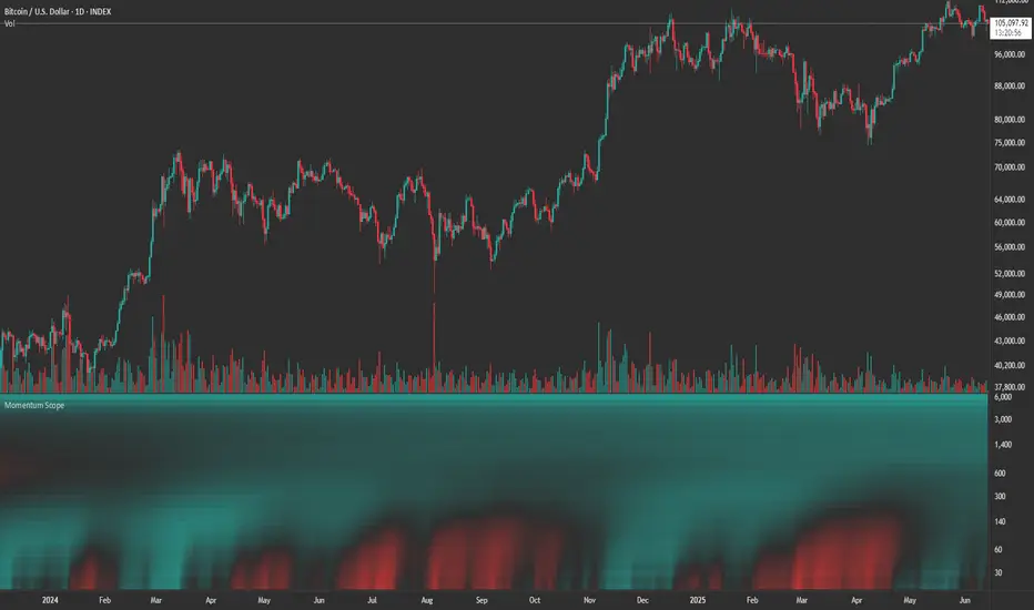
Momentum ScopeOverview
Momentum Scope is a Pine Script™ v6 study that renders a –1 to +1 momentum heatmap across up to 32 lookback periods in its own pane. Using an Augmented Relative Momentum Index (ARMI) and color shading, it highlights where momentum strengthens, weakens, or stays flat over time—across any asset and timeframe.
Key Features
Full-Spectrum Momentum Map : Computes ARMI for 1–32 lookbacks, indexed from –1 (strong bearish) to +1 (strong bullish).
Flexible Scale Gradation : Choose Linear or Exponential spacing, with adjustable expansion ratio and maximum depth.
Trending Bias Control : Apply a contrast-style curve transform to emphasize trending vs. mean-reverting behavior.
Duotone & Tritone Palettes : Select between two vivid color styles, with user-definable hues for bearish, bullish, and neutral momentum.
Compact, Overlay-Free Display : Renders solely in its own pane—keeping your price chart clean.
Inputs & Customization
Scale Gradation : Linear or Exponential spacing of intervals
Scale Expansion : Ratio governing step-size between successive lookbacks
Scale Maximum : Maximum lookback period (and highest interval)
Trending Bias : Curve-transform bias to tilt the –1 … +1 grid
Color Style : Duotone or Tritone rendering modes
Reducing / Increasing / Neutral Colors : Pick your own hues for bearish, bullish, and flat zones
How to Use
Add to Chart : Apply “Momentum Scope” as a separate indicator.
Adjust Scale : For exponential spacing, switch your indicator Y-axis to Logarithmic .
Set Bias & Colors : Tweak Trending Bias and choose a palette that stands out on your layout.
Interpret the Heatmap :
Red tones = weakening/bearish momentum
Green tones = strengthening/bullish momentum
Neutral hues = indecision or flat momentum
Copyright © 2025 MVPMC. Licensed under MIT. For full license see opensource.org
Constance Brown RSI with Composite IndexConstance Brown RSI with Composite Index
Overview
This indicator combines Constance Brown's RSI interpretation methodology with a Composite Index and ATR Distance to VWAP measurement to provide a comprehensive trading tool. It helps identify trends, momentum shifts, overbought/oversold conditions, and potential reversal points.
Key Features
Color-coded RSI zones for immediate trend identification
Composite Index for momentum analysis and divergence detection
ATR Distance to VWAP for identifying extreme price deviations
Automatic divergence detection for early reversal warnings
Pre-configured alerts for key trading signals
How to Use This Indicator
Trend Identification
The RSI line changes color based on its position:
Blue zone (RSI > 50): Bullish trend - look for buying opportunities
Purple zone (RSI < 50): Bearish trend - look for selling opportunities
Gray zone (RSI 40-60): Neutral/transitional market - prepare for potential breakout
The 40-50 area (light blue fill) acts as support during uptrends, while the 50-60 area (light purple fill) acts as resistance during downtrends.
// From the code:
upTrendZone = rsiValue > 50 and rsiValue <= 90
downTrendZone = rsiValue < 50 and rsiValue >= 10
neutralZone = rsiValue > 40 and rsiValue < 60
rsiColor = neutralZone ? neutralRSI : upTrendZone ? upTrendRSI : downTrendRSI
Momentum Analysis
The Composite Index (fuchsia line) provides momentum confirmation:
Values above 50 indicate positive momentum
Values below 40 indicate negative momentum
Crossing above/below these thresholds signals potential momentum shifts
// From the code:
compositeIndexRaw = rsiChange / ta.stdev(rsiValue, rsiLength)
compositeIndex = ta.sma(compositeIndexRaw, compositeSmoothing)
compositeScaled = compositeIndex * 10 + 50 // Scaled to fit 0-100 range
Overbought/Oversold Detection
The ATR Distance to VWAP table in the top-right corner shows how far price has moved from VWAP in terms of ATR units:
Extreme positive values (orange/red): Potentially overbought
Extreme negative values (purple/red): Potentially oversold
Near zero (gray): Price near average value
// From the code:
priceDistance = (close - vwapValue) / ta.atr(atrPeriod)
// Color coding based on distance value
Divergence Trading
The indicator automatically detects divergences between the Composite Index and price:
Bullish divergence: Price makes lower low but Composite Index makes higher low
Bearish divergence: Price makes higher high but Composite Index makes lower high
// From the code:
divergenceBullish = ta.lowest(compositeIndex, rsiLength) > ta.lowest(close, rsiLength)
divergenceBearish = ta.highest(compositeIndex, rsiLength) < ta.highest(close, rsiLength)
Trading Strategies
Trend Following
1. Identify the trend using RSI color:
Blue = Uptrend, Purple = Downtrend
2. Wait for pullbacks to support/resistance zones:
In uptrends: Buy when RSI pulls back to 40-50 zone and bounces
In downtrends: Sell when RSI rallies to 50-60 zone and rejects
3. Confirm with Composite Index:
Uptrends: Composite Index stays above 50 or quickly returns above it
Downtrends: Composite Index stays below 50 or quickly returns below it
4. Manage risk using ATR Distance:
Take profits when ATR Distance reaches extreme values
Place stops beyond recent swing points
Reversal Trading
1. Look for divergences
Bullish: Price makes lower low but Composite Index makes higher low
Bearish: Price makes higher high but Composite Index makes lower high
2. Confirm with ATR Distance:
Extreme readings suggest potential reversals
3. Wait for RSI zone transition:
Bullish: RSI crosses above 40 (purple to neutral/blue)
Bearish: RSI crosses below 60 (blue to neutral/purple)
4. Enter after confirmation:
Use candlestick patterns for precise entry
Place stops beyond the divergence point
Four pre-configured alerts are available:
Momentum High: Composite Index above 50
Momentum Low: Composite Index below 40
Bullish Divergence: Composite Index higher low
Bearish Divergence: Composite Index lower high
Customization
Adjust these parameters to optimize for your trading style:
RSI Length: Default 14, lower for more sensitivity, higher for fewer signals
Composite Index Smoothing: Default 10, lower for quicker signals, higher for less noise
ATR Period: Default 14, affects the ATR Distance to VWAP calculation
This indicator works well across various markets and timeframes, though the default settings are optimized for daily charts. Adjust parameters for shorter or longer timeframes as needed.
Happy trading!

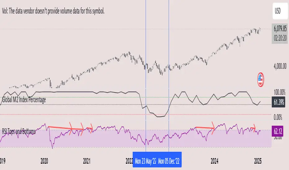
Global M2 Index Percentage### **Global M2 Index Percentage**
**Description:**
The **Global M2 Index Percentage** is a custom indicator designed to track and visualize the global money supply (M2) in a normalized percentage format. It aggregates M2 data from major economies (e.g., the US, EU, China, Japan, and the UK) and adjusts for exchange rates to provide a comprehensive view of global liquidity. This indicator helps traders and investors understand the broader macroeconomic environment, identify trends in money supply, and make informed decisions based on global liquidity conditions.
---
### **How It Works:**
1. **Data Aggregation**:
- The indicator collects M2 data from key economies and adjusts it using exchange rates to calculate a global M2 value.
- The formula for global M2 is:
\
2. **Normalization**:
- The global M2 value is normalized into a percentage (0% to 100%) based on its range over a user-defined period (default: 13 weeks).
- The formula for normalization is:
\
3. **Visualization**:
- The indicator plots the M2 Index as a line chart.
- Key reference levels are highlighted:
- **10% (Red Line)**: Oversold level (low liquidity).
- **50% (Black Line)**: Neutral level.
- **80% (Green Line)**: Overbought level (high liquidity).
---
### **How to Use the Indicator:**
#### **1. Understanding the M2 Index:**
- **Below 10%**: Indicates extremely low liquidity, which may signal economic contraction or tight monetary policy.
- **Above 80%**: Indicates high liquidity, which may signal loose monetary policy or potential inflationary pressures.
- **Between 10% and 80%**: Represents a neutral to moderate liquidity environment.
#### **2. Trading Strategies:**
- **Long-Term Investing**:
- Use the M2 Index to assess global liquidity trends.
- **High M2 Index (e.g., >80%)**: Consider investing in risk assets (stocks, commodities) as liquidity supports growth.
- **Low M2 Index (e.g., <10%)**: Shift to defensive assets (bonds, gold) as liquidity tightens.
- **Short-Term Trading**:
- Combine the M2 Index with technical indicators (e.g., RSI, MACD) for timing entries and exits.
- **M2 Index Rising + RSI Oversold**: Potential buying opportunity.
- **M2 Index Falling + RSI Overbought**: Potential selling opportunity.
#### **3. Macroeconomic Analysis**:
- Use the M2 Index to monitor the impact of central bank policies (e.g., quantitative easing, rate hikes).
- Correlate the M2 Index with inflation data (CPI, PPI) to anticipate inflationary or deflationary trends.
---
### **Key Features:**
- **Customizable Timeframe**: Adjust the lookback period (e.g., 13 weeks, 26 weeks) to suit your trading style.
- **Multi-Economy Data**: Aggregates M2 data from the US, EU, China, Japan, and the UK for a global perspective.
- **Normalized Output**: Converts raw M2 data into an easy-to-interpret percentage format.
- **Reference Levels**: Includes key levels (10%, 50%, 80%) for quick analysis.
---
### **Example Use Case:**
- **Scenario**: The M2 Index rises from 49% to 62% over two weeks.
- **Interpretation**: Global liquidity is increasing, potentially due to central bank stimulus.
- **Action**:
- **Long-Term**: Increase exposure to equities and commodities.
- **Short-Term**: Look for buying opportunities in oversold assets (e.g., RSI < 30).
---
### **Why Use the Global M2 Index Percentage?**
- **Macro Insights**: Understand the broader economic environment and its impact on financial markets.
- **Risk Management**: Identify periods of high or low liquidity to adjust your portfolio accordingly.
- **Enhanced Timing**: Combine with technical analysis for better entry and exit points.
---
### **Conclusion:**
The **Global M2 Index Percentage** is a powerful tool for traders and investors seeking to incorporate macroeconomic data into their strategies. By tracking global liquidity trends, this indicator helps you make informed decisions, whether you're trading short-term or planning long-term investments. Add it to your TradingView charts today and gain a deeper understanding of the global money supply!
---
**Disclaimer**: This indicator is for informational purposes only and should not be considered financial advice. Always conduct your own research and consult with a professional before making investment decisions.
Larry Williams Valuation Index [tradeviZion]Larry Williams Valuation Index
Welcome to the Larry Williams Valuation Index by tradeviZion! This script is an interpretation of Larry Williams' famous WillVal (Valuation) Index, originally developed in 1990 to help traders determine whether a market or asset is overvalued or undervalued. We've extended it to support multiple securities and offer alerts for different valuation levels, helping you make more informed trading decisions.
What is the Valuation Index?
The Valuation Index measures how a security's current price compares to its historical price action. It helps identify whether the security is overvalued (priced too high), undervalued (priced too low), or in a normal range.
This version supports multiple securities and uses valuation parameters to help you assess the relative valuation of three securities simultaneously. It can help you determine the best times to enter (buy) or exit (sell) the market.
Key Features
Multi-Security Analysis: Analyze up to three securities simultaneously to get a broader view of market conditions.
Valuation Levels: Automatically calculate overvaluation and undervaluation levels or set manual levels for consistent analysis.
Custom Alerts: Create custom alerts when securities move between overvalued, undervalued, or normal ranges.
Customizable Table Display: Display a table with valuation values and their status on the chart.
Getting Started
Step 1: Adding the Script to Your Chart
First, add the Larry Williams Valuation Index script to your chart on TradingView. The script is designed to work with any timeframe, but for best results, use weekly or daily timeframes for a longer-term perspective.
Step 2: Configuring Securities
The script allows you to analyze up to three different securities :
Security 1 (Default: DXY)
Security 2 (Default: GC1!)
Security 3 (Default: ZB1!)
You can enable or disable each security individually.
Custom Timeframe Option: You have the option to select a custom timeframe for analysis. This allows you to see whether the security is overvalued or undervalued in lower or higher timeframes. Note that this feature is experimental and has not been extensively tested. Larry Williams originally used the weekly timeframe to determine if a stock was overvalued or undervalued. By default, the indicator compares the current price with the security based on the selected timeframe, except if you choose to use a custom timeframe.
Pro Tip : New users can start with the default securities to understand the concept before using other assets.
Step 3: Valuation Index Settings
Short EMA Length : This is the short-term average used for calculations. A lower value makes it more responsive to recent price changes.
Long EMA Length : This is the long-term average, used to smooth the valuation over time.
Valuation Length (Default: 156) : Represents approximately three years of daily bars (as recommended by Larry Williams).
How is the Valuation Index Calculated?
The valuation calculation is done using a method called WVI (WillVal Index), which compares the current price of a security to the price of another correlated security. Here’s a step-by-step explanation:
1. Data Collection: The script takes the closing price of the security you are analyzing and the closing price of the correlated security.
2. Ratio Calculation : The ratio of the two prices is calculated:
Price Ratio = (Price of your security) / (Price of correlated security) * 100.
This ratio helps determine how expensive or cheap your security is compared to the correlated one.
3. Exponential Moving Averages (EMAs) : The price ratio is used to calculate short-term and long-term EMAs (Exponential Moving Averages). EMAs are used to create smooth lines that represent the average price of a security over a specific period of time, with more weight given to recent data. By calculating both short-term and long-term EMAs, we can identify the trend direction and how the security is performing compared to its historical averages.
4. Valuation Index Calculation:
The Valuation Index is calculated as the difference between the short-term EMA and the long-term EMA. This difference helps to determine if the security is currently overvalued or undervalued:
A positive value indicates that the price is above its longer-term trend, suggesting potential overvaluation.
A negative value indicates that the price is below its longer-term trend, suggesting potential undervaluation.
5. Normalization:
To make the valuation easier to interpret, the calculated valuation index is then normalized using the highest and lowest values over the selected valuation length (e.g., 156 bars).
This normalization process converts the index into a percentage between 0 and 100, where higher values indicate overvaluation and lower values indicate undervaluation.
Step 4: Understanding Valuation Levels
The valuation levels indicate whether a security is currently undervalued, overvalued, or in a normal range.
Manual Levels : You can manually set the overvaluation and undervaluation thresholds (default is 85 for overvalued and 15 for undervalued).
Auto Levels : The script can automatically calculate these levels based on recent price action, allowing you to adapt to changing market conditions.
Auto Levels Calculation Explained:
The Auto Levels are calculated by taking the average of the valuation indices for all three securities (e.g., index1, index2, and index3).
The script then looks at the highest and lowest values of this average over a selected number of recent bars (e.g., 50 bars).
The overvaluation level is determined by taking the highest value and multiplying it by a multiplier (e.g., 5). Similarly, the undervaluation level is calculated using the lowest value and the multiplier.
These dynamic levels adjust according to recent price action, providing an adaptive approach to identifying overvalued and undervalued conditions.
Step 5: How to Use the Script to Make Trading Decisions
For new users, here's a step-by-step trading strategy you can use with the Valuation Index:
1. Identify Undervalued Opportunities
When two or more securities are in the undervalued range (below 15 for manual or below automatically calculated undervalue levels), wait for at least two of these securities to turn from undervalued to normal .
This transition indicates a potential buy opportunity .
2. Buying Signal
When at least two securities transition from undervalued to normal, you can consider buying the asset.
This indicates that the market may be recovering from undervalued conditions and could be moving into a growth phase.
3. Selling Signal
Exit when the price high closes below the EMA 21 (21-day exponential moving average).
Alternatively, if the valuation index reaches overvalued levels (above 85 manually or auto-calculated), wait for it to drop back to normal . This can be another point to exit the trade .
You can also use any other sell condition based on your r isk management strategy .
Alerts for Valuation Levels
The script includes alerts to notify you of changing market conditions:
To activate these alerts, follow these steps, referring to the provided screenshot with detailed steps:
1. Enable Alerts : Click on the settings gear icon on the script title in your chart. In the settings menu, scroll to the section labeled Alerts Settings .
Enable Alerts by checking the Enable Alerts box.
Set the Required Securities for Alert (default is 2 securities).
Choose the Alert Frequency : Selecting Once Per Bar Close will trigger alerts only at the close of each bar, ensuring you receive confirmed signals rather than potentially noisy intermediate signals.
2. Select Alert Type : Choose the type of alert you want to activate, such as Alert on Overvalued, Alert on Undervalued, Alert on Over to Normal , or Alert on Under to Normal .
3. Save Settings : Click OK to save your alert settings.
4. Add Alert on Indicator : Click the "..." (More button) next to the indicator name on the chart and select " Add alert on tradeviZion - WillVal ".
5. Create Alert : In the Create Alert window:
Set Condition to tradeviZion - WillVal .
Ensure Any alert() function call is selected.
Set the Alert Name and select your Expiration preferences.
6. Set Notification Preferences : Go to the Notifications tab and select how you want to receive notifications, such as via app notification, toast notification, email , or sound alert . Adjust these preferences to best suit your needs.
7. Click Create : Finally, click Create to activate the alert.
These alerts will help you stay informed about key market conditions and take action accordingly, ensuring you do not miss critical trading opportunities.
Understanding the Table Display
The script includes an interactive table on the chart to show the valuation status of each security:
Security : The name of the security being analyzed.
Value : The current valuation index value.
Status : Indicates whether the security is overvalued, undervalued , or in a normal range.
Color: Displays a color code for easy identification of status:
Red for overvalued.
Green for undervalued.
Other colors represent normal valuation levels.
Empowering Messages : Motivational messages are displayed to encourage disciplined trading. These messages will change periodically, helping keep a positive trading mindset.
Acknowledgment
This tool builds upon the foundational work of Larry Williams, who developed the WillVal (Valuation) Index concept. It also incorporates enhancements to extend multi-security analysis, valuation normalization, and advanced alerting features, providing a more versatile and powerful indicator. The Larry Williams Valuation Index [ tradeviZion ] helps traders make informed decisions by assessing overvalued and undervalued conditions for multiple securities simultaneously.
Note : Always practice proper risk management and thoroughly test the indicator to ensure it aligns with your trading strategy. Past performance is not indicative of future results.
Trade smarter with TradeVizion—unlock your trading potential today!

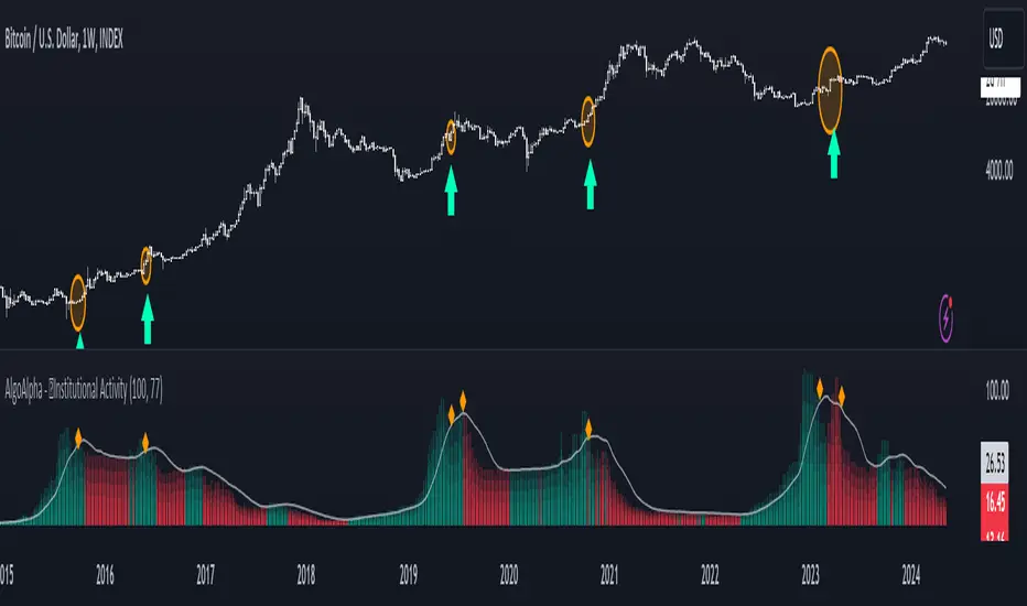
Institutional Activity Index [AlgoAlpha]🌟 Introducing the Institutional Activity Index by AlgoAlpha 🌟
Welcome to a powerful new indicator designed to gauge institutional trading activity! This cutting-edge tool combines volume analysis with price movement to derive a unique index that shines a spotlight on potential institutional moves in the market. 🎯📈
Key Features:
🔍 Normalization Period : Adjust the look-back period for normalization to tailor the sensitivity to your trading strategy.
📊 Moving Average Types : Choose from SMA, HMA, EMA, RMA, WMA, or VWMA to smooth the index and pinpoint trends.
🌈 Color-Coded Trends : Instant visual feedback on index trend direction with customizable up and down colors.
🔔 Alerts : Set alerts for when the index shows increasing activity, decreasing activity, or has reached a peak.
Quick Guide to Using the Institutional Activity Index:
1. 📝 Add the Indicator: Add the indicator to favorites. Adjust the normalization period, MA type, and peak detection settings to match your trading style.
2. 📈 Market Analysis: Similar to volume that reflects the amount of collective trading activity, this index reflects an estimate of the amount of trading activity by institutions. A higher value means that institutions are trading the asset more, this can mean selling or buying as the indicator does not indicate direction . Look out for peak signals, which may indicate that institutions have already secured positions in preparation for a move in price.
3. 🔔 Set Alerts: Enable alerts to notify you when there is a significant change in the activity levels or a new peak is detected, allowing for timely decisions without constant monitoring.
How It Works: 🛠
It is common knowledge that institutions trade with high amounts of capital, but employ tactics so as to not move the price significantly when entering on positions. This can be done by entering in times of high liquidity so that when an institution buys, there are enough sellers to cancel out the price movements and prevent a huge pump in price and vice versa. The Institutional Activity Index calculates liquidity by measuring the volume relative to the price range (close-open). This value is smoothed using median and a user defined moving average type and period, enhancing its clarity. If normalization is enabled, the index is adjusted relative to its range over a user-defined period, making the data comparable across different conditions.
Embrace this innovative tool to enhance your trading insights and strategies! 🚀✨
[BT] NedDavis Series: CPI Minus 5-Year Moving Average🟧 GENERAL
The script works on the Monthly Timeframe and has 2 main settings (explained in FEATURES ). It uses the US CPI data, reported by the Bureau of Labour Statistics.
🔹Functionality 1: The main idea is to plot the distance between the CPI line and the 5 year moving average of the CPI line. This technique in mathematics is called "deviation from the moving average". This technique is used to analyse how has CPI previously acted and can give clues at what it might do in the future. Economic historians use such analysis, together with specific period analysis to predict potential risks in the future (see an example of such analysis in HOW TO USE section. The mathematical technique is a simple subtraction between 2 points (CPI - 5yr SMA of CPI).
▶︎Interpretation for deviation from a moving average:
Positive Deviation: When the line is above its moving average, it indicates that the current value is higher than the average, suggesting potential strength or bullish sentiment.
Negative Deviation: Conversely, when the line falls below its moving average, it suggests weakness or bearish sentiment as the current value is lower than the average.
▶︎Applications:
Trend Identification: Deviations from moving averages can help identify trends, with sustained deviations indicating strong trends.
Reversal Signals: Significant deviations from moving averages may signal potential trend reversals, especially when combined with other technical indicators.
Volatility Measurement: Monitoring the magnitude of deviations can provide insights into market volatility and price movements.
Remember the indicator is applying this only for the US CPI - not the ticker you apply the indicator on!
🔹Functionality 2: It plots on a new pane below information about the Consumer Price Index. You can also find the information by plotting the ticker symbol USACPIALLMINMEI on TradingView, which is a Monthly economic data by the OECD for the CPI in the US. The only addition you would get from the indicator is the plot of the 5 year Simple Moving Average.
🔹What is the US Consumer Price Index?
Measures the change in the price of goods and services purchased by consumers;
Traders care about the CPI because consumer prices account for a majority of overall inflation. Inflation is important to currency valuation because rising prices lead the central bank to raise interest rates out of respect for their inflation containment mandate;
It is measured as the average price of various goods and services are sampled and then compared to the previous sampling.
Source: Bureau of Labor Statistics;
FEATURES OF INDICATOR
1) The US Consumer Price Index Minus the Five Year Moving Average of the same.
As shown on the picture above and explained in previous section. Here a more detailed view.
2) The actual US Consumer Price Index (Annual Rate of change) and the Five year average of the US Consumer Price Index. Explained above and shown below:
To activate 2) go into settings and toggle the check box.
HOW TO USE
It can be used for a fundamental analysis on the relationship between the stock market, the economy and the Feds decisions to hike or cut rates, whose main mandate is to control inflation over time.
I have created this indicator to show my analysis in this idea:
What does a First Fed Rate cut really mean?
CREDITS
I have seen such idea in the past posted by the institutional grade research of NedDavis and have recreated it for the TradingView platform, open-source for the community.

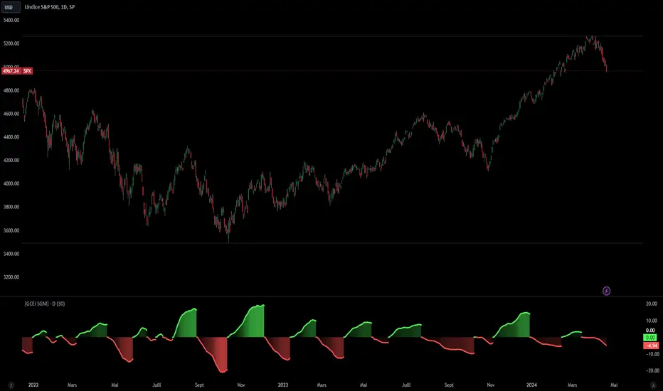
[Global Contraction Expansion Index SGM]Script Features
Dynamic Period Choice: The user can adjust the calculation period (period) for relative performance, allowing flexibility according to specific market analysis needs.
Sector Selection: The script takes into account different economic sectors through well-known ETFs like QQQ (technology), XLF (financial), XLY (consumer discretionary), XLV (healthcare), XLI (industrial) and XLE (energy). This diversification helps gain a general overview of economic health across different market segments.
Relative Performance Calculation: For each sector, the script calculates the relative performance using a simple moving average (SMA) of the price change over the specified period. This helps identify price trends adjusted for normal market fluctuations.
GCEI Index: The GCEI Index is calculated as the average of the relative performance of all sectors, multiplied by 100 to express it as a percentage. This provides an overall indicator of sectoral economic performance.
Crossover Signals: The script detects and marks points where the overall index (GCEI) crosses its own exponential moving average (emaGCEI), indicating potential changes in the overall trend of market performance.
Visualization: Results are visualized through graphs, where positive and negative regions are colored differently. Fills between the zero line and the index curves make it easy to see periods of contraction or expansion
When this index diverges from the SP500, it may be a sign that the technology sector is outperforming other sectors.
Enhanced McClellan Summation Index
The Enhanced McClellan Summation Index (MSI) is a comprehensive tool that transforms the MSI indicator with Heikin-Ashi visualization, offering improved trend analysis and momentum insights. This indicator includes MACD and it's histogram calculations to refine trend signals, minimize false positives and offer additional momentum analysis.
Methodology:
McClellan Summation Index (MSI) -
The MSI begins by calculating the ratio between advancing and declining issues in the specified index.
float decl = 𝘐𝘯𝘥𝘪𝘤𝘦 𝘥𝘦𝘤𝘭𝘪𝘯𝘪𝘯𝘨 𝘪𝘴𝘴𝘶𝘦𝘴
float adv = 𝘐𝘯𝘥𝘪𝘤𝘦 𝘢𝘥𝘷𝘢𝘯𝘤𝘪𝘯𝘨 𝘪𝘴𝘴𝘶𝘦𝘴
float ratio = (adv - decl) / (adv + decl)
It then computes a cumulative sum of the MACD (the difference between a 19-period EMA and a 39-period EMA) of this ratio. The result is a smoothed indicator reflecting market breadth and momentum.
macd(float r) =>
ta.ema(r, 19) - ta.ema(r, 39)
float msi = ta.cum(macd(ratio))
Heikin-Ashi Transformation -
Heikin-Ashi is a technique that uses a modified candlestick formula to create a smoother representation of price action. It averages the open, close, high, and low prices of the current and previous periods. This transformation reduces noise and provides a clearer view of trends.
type bar
float o = open
float h = high
float l = low
float c = close
bar b = bar.new()
float ha_close = math.avg(b.o, b.h, b.l, b.c)
MACD and Histogram -
The Enhanced MSI incorporates MACD and histogram calculations to provide additional momentum analysis and refine trend signals. The MACD represents the difference between the 12-period EMA and the 26-period EMA of the MSI. The histogram is the visual representation of the difference between the MACD and its signal line.
Options:
Index Selection - Choose from TVC:NYA , NASDAQ:NDX , or TVC:XAX to tailor the MSI-HA to the desired market index.
MACD Settings - Adjust the parameters for the MACD calculation to fine-tune the indicator's responsiveness.
Ratio Multiplier - Apply scaling to the MSI to suit different market conditions and indices.
Benefits of Heikin-Ashi -
Smoothed Trends - Heikin-Ashi reduces market noise, providing a more apparent and smoothed representation of trends.
Clearer Patterns - Candlestick patterns are more distinct, aiding in the identification of trend reversals and continuations.
Utility and Use Cases:
Trend & Momentum Analysis - Utilize the tool's Heikin-Ashi visualization for clearer trend identification in confluence with it's MACD and histogram to gain additional insights into the strength and direction of trends, while filtering out potential false positives.
Breadth Analysis - Explore market breadth through the MSI's cumulative breadth indicator, gauging the overall health and strength of the underlying market.
- Alerts Setup Guide -
The Enhanced MSI is a robust indicator that combines the breadth analysis of the McClellan Summation Index with the clarity of Heikin-Ashi visualization and additional momentum insights from MACD and histogram calculations. Its customization options make it adaptable to various indices and market conditions, offering traders a comprehensive tool for trend and momentum analysis.
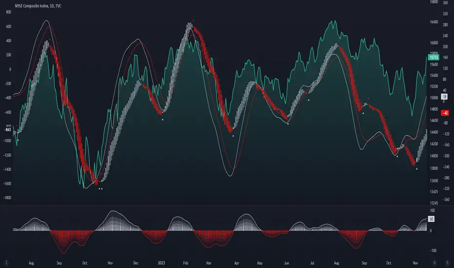
RSIOMA with Volume Index ConfirmationThis indicator is called "RSIOMA with Volume Index Confirmation". It is a technical analysis tool that plots buy and sell signals on a chart based on the Relative Strength Index (RSI) and the Negative Volume Index (NVI) and Positive Volume Index (PVI) indicators.
The indicator has the following input parameters:
- RSI Length: determines the number of periods used to calculate the RSI. Default value is 14.
- Overbought Level: determines the RSI level at which a security is considered overbought. Default value is 70.
- Oversold Level: determines the RSI level at which a security is considered oversold. Default value is 30.
- NVI Length: determines the number of periods used to calculate the Negative Volume Index. Default value is 255.
- PVI Length: determines the number of periods used to calculate the Positive Volume Index. Default value is 255.
The indicator calculates the RSI using the RSI Length input parameter and the close price of the security. It also calculates the NVI and PVI by looping through the volume data and the close price data of the security over the specified periods.
The indicator then uses the RSI, NVI, and PVI to determine buy and sell signals. A bearish divergence signal is generated when the RSI from one period ago is greater than the Overbought Level, the current RSI is less than the Overbought Level, and the close price from one period ago is greater than the current close price. A bullish divergence signal is generated when the RSI from one period ago is less than the Oversold Level, the current RSI is greater than the Oversold Level, and the close price from one period ago is less than the current close price. A sell signal is generated when a bearish divergence signal occurs and the current NVI is less than the previous NVI value. A buy signal is generated when a bullish divergence signal occurs and the current PVI is greater than the previous PVI value.
The indicator plots the buy and sell signals on the chart as green and red triangles, respectively. The "overlay=true" parameter in the indicator function indicates that the signals are plotted on top of the security's price chart.

Smart Disparity IndexThe Smart Disparity Index (SDI) is an optimized version of the Disparity Index indicator invented by Steve Nison (book "Beyond Candlesticks").
According to Steve Nison, "The disparity index (or disparity ratio), compares, as a percentage, the latest close to a chosen moving average", which means that the indicator gives the difference in % between the closing price and a simple moving average.
The calculation formula is therefore as follows:
Disparity Index = 100 x (closing_price - simple_moving_average) / simple_moving_average
In order to optimize the calculation, I replaced the closing price with the 6-period exponential moving average (EMA6) which, according to many years of experience, allows prices to be smoothed by eliminating excesses.
Formula for calculating the Smart Disparity Index:
SDI = 100 x (EMA6 - simple_moving_average) / simple_moving_average
The provided script displays the SDI for the 20, 50, 100 and 200 periods.
From my point of view, I recommend using the SDI50 as a priority:
SDI50 = 100 x (EMA6 - SMA50) / SMA50
In the chart, we can see the SDI50 (in purple) is on a long-term support (in green), this indicates a probability of a Bitcoin rise in the coming months.
The SDI can also be used as a momentum type indicator.

Relative Index StrengthThis script shows relative strength of custom stock compared to Index. It is helpful in detecting how strongly a stock is performing when compared to an Index.
When the index is falling but the custom stock is rising, indicator shows this in red with its relative strength compared to index, indicating the stock is moving strongly against market trend.
When the index and the custom stock are moving in same direction, indicator remains neutral, indicating the stock is aligned with the market trend.
VIX - SKEW DivergenceThe CBOE VIX is a well-known index representing market expectations for volatility over the next 30 days.
The CBOE SKEW is an index reflecting the perceived tail risk over the next 30 days.
When the SKEW rises over a certain level (~140/150), that means investors are hedging their exposure with options, because they are worried about an incoming market crash or a "black swan". If that happens when the VIX is very low and apparently there is no uncertainty, this can warn of a sudden change in direction of the market. You will see for yourself that an increasing divergence often anticipates a sharp fall of leading stock indexes, usually within two to four months.
This is probably not very relevant for the short-term trader but mid/long-term traders and market analysts may find it useful to clearly visualize the extent of the distance between the VIX and the SKEW. For that reason, I wrote this highly customizable script with which you can plot the two indexes and fill the space within them with a color gradient to highlight the maximum and minimum divergence. Additionally, you can fill the beneath VIX area with four different colors. It is also possible to plot the divergence value itself, so if you want you can draw trendlines and support/resistance levels on it.
Please note that the divergence per se doesn't predict anything and it's meant to be used synergistically with other technical analysis tools.
More informations here:
www.cboe.com
www.cboe.com

TASC 2022.08 Trading The Fear Index█ OVERVIEW
TASC's August 2022 edition of Traders' Tips includes an article by Markos Katsanos titled "Trading The Fear Index". This script implements a trading strategy called the “daily long/short trading system for volatility ETFs” presented in this article.
█ CONCEPTS
This long-term strategy aims to capitalize on stock market volatility by using exchange-traded funds (ETFs or ETNs) linked to the VIX index.
The strategy rules (see below) are based on a combination of the movement of the Cboe VIX index, the readings of the stochastic oscillator applied to the SPY ETF relative to the VIX, and a custom indicator presented in the article and called the correlation trend . Thus, they are not based on the price movement of the traded ETF itself, but rather on the movement of the VIX and of the S&P 500 index. This allows the strategy to capture most of the spikes in volatility while profiting from the long-term time decay of the traded ETFs.
█ STRATEGY RULES
Long rules
Rising volatility: The VIX should rise by more than 50% in the last 6 days.
Trend: The correlation trend of the VIX should be 0.8 or higher and also higher than yesterday's value.
VIX-SPY relative position: The 25-day and 10-day VIX stochastics should be above the 25-day and 10-day SPY stochastics respectively. In addition, the 10-day stochastic of the VIX should be above its yesterday's value.
Long positions are closed if the 10-day stochastic of the SPY rises above the 10-day stochastic of the VIX or falls below the yesterday's value.
Short rules
Declining volatility: The VIX should drop over 20% in the last 6 days and should be down during the last 3 days.
VIX threshold: The VIX should spend less than 35% of time below 15.
VIX-SPY relative position: The 10-day VIX stochastic should be below the 10-day SPY stochastic. In addition, the 10-day SPY stochastic should be higher than the yesterday's value.
Long positions are closed if the first two Long rules are triggered (Rising volatility and Trend).
The script allows you to display the readings of the indicators used in the strategy rules in the form of oscillator time series (as in the preview chart) and/or in the form of a table.

Market breadth Percentage of stocks above MA of various indexesPercentage of stock above moving average is a common market breadth indicator. This script can show multiple lines of percentage of stock above different moving average (5,20,50,100,150,200) of different US indexes.

Bollinger Bands Money Flow IndexThis script embodies the application of the Bollinger Band and Money Flow Index in John A. Bollinger's book "Bollinger on Bollinger Bands."
"Bollinger on Bollinger Bands" suggests a relatively method of analysis by applying the Bollinger Band to an indicator.
Here's one of the indicators, Money Flow Index.
Money Flow Index is an indicator of overbuying and overselling by reflecting the volume of transactions.
"Bollinger on Bollinger Bands" suggests using the Bollinger Band to create relative top and bottom lines for various indicators, such as Money Flow Index.
Original Money Flow Index is considered to be over-purchased if it is more than 80% and over-selling if it is less than 20%.
But if you put a bolinger band on it, you can set the standard for higher or lower over-selling and over-selling in a sustained bullish, bearish market.
This script uses the following values as the default values as recommended by "Bollinger on Bollinger Bands".
Money Flow Index for 10 days.
a bollinger band of forty days
standard deviation of 2
The above values are suitable for most stocks and markets, but sometimes there is too much or too little data inside the Bollinger Band.
It is recommended to modify each value little by little to adjust 85% to 90% of the total data to fit inside the Bollinger Band.
If the value is higher than the top line, it is considered over-purchased, and a red background color appears.
If the bottom line is crossed down, it is considered over-sold and the green background color appears.
