Strat Reversal MTF TableStrat Reversal MTF Table — Your Complete Multi-Timeframe Strat Command Center
Take your Strat trading to the next level with an indicator that shows every reversal, on every timeframe, in one powerful visual dashboard.
Designed for traders who demand speed, clarity, and full Strat alignment, the Strat Reversal MTF Table instantly identifies all major bullish and bearish reversal patterns:
Bullish Patterns
2-1-2
3-1-2
1-3-2
3-2-2
Bearish Patterns
2-1-2
3-1-2
1-3-2
3-2-2
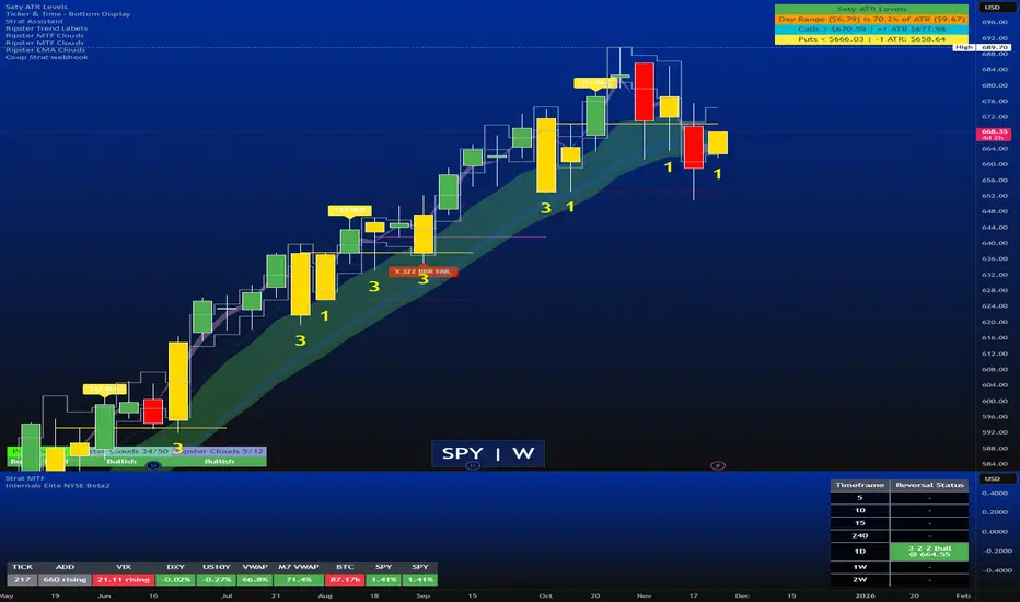
Each signal is displayed with:
Clear pattern name (e.g., “2-1-2 Bull”)
Automatic trigger price
Timeframe label
Color-coded background (Bullish / Bearish / Neutral)
Whether you trade options, equities, futures, or crypto, this indicator makes it effortless to see what’s flipping — and where the strongest setups are emerging.
🔥 Key Features
📊 Multi-Timeframe Scanning (1 min → Daily)
Monitor 7 customizable timeframes at once.
From scalping to swing trading, you always know which timeframe is turning.
⚡ Real-Time OR Close-Confirmed Logic
Choose your style:
Realtime (Wick Mode) → Fast entries
Close-Confirmed → Stronger validation
Ideal for traders who want precision on any timeframe.
🎨 Clean & Customizable Dashboard
Move the table anywhere on the chart
Adjust text size
Choose your own colors
Lightweight and non-intrusive
A perfect blend of simplicity and power.
📩 Instant Alerts, Built In
Get notified instantly when:
Any timeframe reverses
A specific timeframe flips
Multiple reversals fire across the stack
The indicator works great with TradingView’s push notifications, email, and webhooks.
🎯 What This Helps You Do
✔ Catch Strat reversals as they happen
✔ Quickly spot full-timeframe alignment
✔ Improve your entries for options plays
✔ Avoid chop by reading higher-timeframe intent
✔ Trade more confidently with automated trigger levels
This indicator is built for Strat traders who want to trade smarter, faster, and cleaner.
✨ Perfect For
Strat Traders
Options Traders
Futures Scalpers
Intraday & Swing Traders
Quant/Algo-inspired traders
Anyone following Rob Smith’s methodology
مؤشر Pine Script®