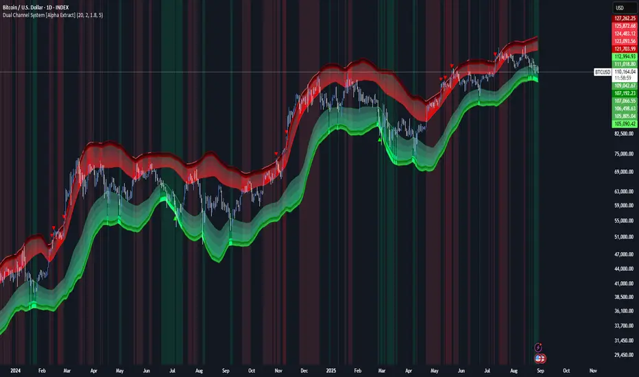
ETF Leverage VerificationDo leveraged ETFs really return what they promise?
Do they return the exact 2x or 3x? Or a slightly different multiple?
How much do they deviate from the promised leverage multiples?
Do these deviations impact investors in a positive or negative manner?
These are the questions that I want to answer with this indicator.
The ETF Leverage Verification indicator challenges the conventional understanding of leveraged ETFs by measuring how they actually perform versus their theoretical targets.
Instead of assuming leveraged ETFs perfectly track their target multiple, this indicator quantifies the real-world behavior by comparing the expected returns versus the actual results on every trading day.
Key Features
Measures actual versus expected performance of leveraged ETFs
Tracks deviation patterns across thousands of trading days
Identifies asymmetric behavior in up versus down markets
Quantifies beneficial "cushioning effect" during market declines
Provides statistical summary of performance patterns
Works with any leverage factor (2x, 3x, -1x, etc.)
Compatible with all leveraged ETFs (equity, bond, commodity, volatility)
How to Use the Indicator
Enter the Expected Leverage Factor (default: 2.0)
Select the Base Asset (underlying index, e.g., SPX)
Select the Leveraged Asset (leveraged ETF, e.g., SSO)
Understanding the Results
Green markers: Days when the ETF outperformed its expected multiple
Red markers: Days when the ETF underperformed its expected multiple
Data Table:
Positive Deviations: Count of days with better-than-expected performance
Negative Deviations: Count of days with worse-than-expected performance
Avg Deviation: Average magnitude of deviation from expected returns
Frequency Skew: Difference between beneficial deviations in down vs. up markets
Impact: Overall assessment of pattern benefit to investors
Summary Label:
Percentage of positive deviations in up and down markets
Total sample size for statistical significance
Key Patterns to Look For
Positive Deviation in Negative Days:
This occurs when a leveraged ETF falls less than expected during market declines. For example, if SPX falls 1% and a 2x ETF falls only 1.8% (instead of the expected 2%), this creates a +0.2% deviation. This pattern is beneficial as it provides downside protection.
Negative Deviation in Positive Days:
This happens when a leveraged ETF rises less than expected during market advances. For example, if SPX rises 1% and a 2x ETF rises only 1.9% (instead of the expected 2%), this creates a -0.1% deviation. This pattern reduces upside performance.
Frequency Skew:
The most critical metric that measures how much more frequently beneficial deviations occur in down markets compared to up markets. A higher positive skew indicates a stronger asymmetric pattern that helps long-term performance.
Mathematical Background
The indicator computes the deviation between expected and actual performance:
Deviation = Actual Return - Expected Return
Where:
Expected Return = Base Asset Return × Leverage Factor
The deviation is then categorized into four possible outcomes:
Positive deviation on positive market days
Negative deviation on positive market days
Positive deviation on negative market days
Negative deviation on negative market days
In short, more positive deviations are good for investors.
Please feel free to criticize. I'm happy to improve the indicator.
ابحث في النصوص البرمجية عن "pattern"
Flexible Reversal DetectorFlexible Reversal Detector
An advanced, fully customizable analytical tool designed to identify local trend reversal zones based on candlestick formations. Users have full control over all logic parameters, making it adaptable to different trading styles and preferences.
Key Features
Adjustable maximum pattern length (number of candles)
Customizable body size ratios for initial, middle, and final candles
Configurable minimum price movement (in %) required before a pattern is considered valid
Colored horizontal lines showing the full length of the pattern – helpful in identifying structure, potential support/resistance zones
Optional volume filter – the volume of the final candle is compared to a volume SMA; multiplier can be adjusted (e.g. 1 = equal to average, 0.8 = 80% of average)
Logic Overview
U Pattern
Each bearish candle is treated as a potential start of a reversal pattern.
Subsequent candles, if small enough and within defined thresholds, form the middle part of the structure.
When a bullish candle with a sufficiently large body appears, it is marked as the final candle of the pattern.
The pattern is considered valid if it was preceded by a defined percentage price drop and – optionally – if the volume condition was met.
∩ Pattern
Each bullish candle may act as the initial candle of a potential reversal pattern in the opposite direction.
Following smaller candles form the middle part, as long as they meet the defined criteria.
The appearance of a strong bearish candle marks the end of the formation.
If this pattern is preceded by a certain price increase (and optionally meets the volume filter), it is highlighted on the chart.
Note: On markets with low volatility or on lower timeframes, it is recommended to reduce the percentage thresholds for signal detection. For more dynamic price action or higher timeframes, consider increasing them accordingly.
Visualization
The final candle of the pattern is marked visually on the chart (depending on direction)
Colored horizontal lines indicate the full span of the pattern – from initial to final candle
GStrategy 1000Pepe 15mTrend Following Candlestick Strategy with EMA Filter and Exit Delay
Strategy Concept
This strategy combines candlestick patterns with EMA trend filtering to identify high-probability trade entries, featuring:
Entry Signals: Hammer and Engulfing patterns confirmed by EMA trend
Trend Filter: Fast EMA (20) vs Slow EMA (50) crossover system
Risk Management: 5% stop-loss + 1% trailing stop
Smart Exit: 2-bar delay after exit signals to avoid whipsaws
Key Components
Trend Identification:
Uptrend: Fast EMA > Slow EMA AND rising
Downtrend: Fast EMA < Slow EMA AND falling
Entry Conditions:
pinescript
// Bullish Entry (Long)
longCondition = (Hammer OR Bullish Engulfing)
AND Uptrend
AND no existing position
// Bearish Entry (Short)
shortCondition = Bearish Engulfing
AND Downtrend
AND no existing position
Exit Mechanics:
Primary Exit: EMA crossover (Fast crosses Slow)
Delayed Execution: Waits 2 full candles after signal
Emergency Exits:
5% fixed stop-loss
1% trailing stop
Visual Dashboard:
Colored EMA lines (Blue=Fast, Red=Slow)
Annotated candlestick patterns
Background highlighting for signals
Distinct markers for entries/exits
Unique Features
Pattern Recognition:
Enhanced Hammer detection (strict body/wick ratios)
Multi-candle engulfing confirmation
Trend-Confirmation:
Requires price and EMA alignment
Filters counter-trend patterns
Exit Optimization:
pinescript
// Delay implementation
if exit_signal_triggered
counter := 2 // Start countdown
else if counter > 0
counter -= 1 // Decrement each bar
exit_trade = (counter == 1) // Execute on final bar
Risk Parameters
Parameter Value Description
Stop Loss 5% Fixed risk per trade
Trailing Stop 1% Locks in profits
Exit Delay 2 bars Reduces false exits
Position Size 100% No pyramiding
Visualization Examples
🟢 Green Triangle: Bullish entry
🔴 Red Triangle: Bearish entry
⬇️ Blue X: Long exit (after delay)
⬆️ Green X: Short exit (after delay)
🎯 Pattern Labels: Identifies hammer/engulfing
Recommended Use
Timeframes: 1H-4H (reduces noise)
Markets: Trend-prone assets (FX, indices)
Best Conditions: Strong trending markets
Avoid: Choppy/Ranging markets
Langlands-Operadic Möbius Vortex (LOMV)Langlands-Operadic Möbius Vortex (LOMV)
Where Pure Mathematics Meets Market Reality
A Revolutionary Synthesis of Number Theory, Category Theory, and Market Dynamics
🎓 THEORETICAL FOUNDATION
The Langlands-Operadic Möbius Vortex represents a groundbreaking fusion of three profound mathematical frameworks that have never before been combined for market analysis:
The Langlands Program: Harmonic Analysis in Markets
Developed by Robert Langlands (Fields Medal recipient), the Langlands Program creates bridges between number theory, algebraic geometry, and harmonic analysis. In our indicator:
L-Function Implementation:
- Utilizes the Möbius function μ(n) for weighted price analysis
- Applies Riemann zeta function convergence principles
- Calculates quantum harmonic resonance between -2 and +2
- Measures deep mathematical patterns invisible to traditional analysis
The L-Function core calculation employs:
L_sum = Σ(return_val × μ(n) × n^(-s))
Where s is the critical strip parameter (0.5-2.5), controlling mathematical precision and signal smoothness.
Operadic Composition Theory: Multi-Strategy Democracy
Category theory and operads provide the mathematical framework for composing multiple trading strategies into a unified signal. This isn't simple averaging - it's mathematical composition using:
Strategy Composition Arity (2-5 strategies):
- Momentum analysis via RSI transformation
- Mean reversion through Bollinger Band mathematics
- Order Flow Polarity Index (revolutionary T3-smoothed volume analysis)
- Trend detection using Directional Movement
- Higher timeframe momentum confirmation
Agreement Threshold System: Democratic voting where strategies must reach consensus before signal generation. This prevents false signals during market uncertainty.
Möbius Function: Number Theory in Action
The Möbius function μ(n) forms the mathematical backbone:
- μ(n) = 1 if n is a square-free positive integer with even number of prime factors
- μ(n) = -1 if n is a square-free positive integer with odd number of prime factors
- μ(n) = 0 if n has a squared prime factor
This creates oscillating weights that reveal hidden market periodicities and harmonic structures.
🔧 COMPREHENSIVE INPUT SYSTEM
Langlands Program Parameters
Modular Level N (5-50, default 30):
Primary lookback for quantum harmonic analysis. Optimized by timeframe:
- Scalping (1-5min): 15-25
- Day Trading (15min-1H): 25-35
- Swing Trading (4H-1D): 35-50
- Asset-specific: Crypto 15-25, Stocks 30-40, Forex 35-45
L-Function Critical Strip (0.5-2.5, default 1.5):
Controls Riemann zeta convergence precision:
- Higher values: More stable, smoother signals
- Lower values: More reactive, catches quick moves
- High frequency: 0.8-1.2, Medium: 1.3-1.7, Low: 1.8-2.3
Frobenius Trace Period (5-50, default 21):
Galois representation lookback for price-volume correlation:
- Measures harmonic relationships in market flows
- Scalping: 8-15, Day Trading: 18-25, Swing: 25-40
HTF Multi-Scale Analysis:
Higher timeframe context prevents trading against major trends:
- Provides market bias and filters signals
- Improves win rates by 15-25% through trend alignment
Operadic Composition Parameters
Strategy Composition Arity (2-5, default 4):
Number of algorithms composed for final signal:
- Conservative: 4-5 strategies (higher confidence)
- Moderate: 3-4 strategies (balanced approach)
- Aggressive: 2-3 strategies (more frequent signals)
Category Agreement Threshold (2-5, default 3):
Democratic voting minimum for signal generation:
- Higher agreement: Fewer but higher quality signals
- Lower agreement: More signals, potential false positives
Swiss-Cheese Mixing (0.1-0.5, default 0.382):
Golden ratio φ⁻¹ based blending of trend factors:
- 0.382 is φ⁻¹, optimal for natural market fractals
- Higher values: Stronger trend following
- Lower values: More contrarian signals
OFPI Configuration:
- OFPI Length (5-30, default 14): Order Flow calculation period
- T3 Smoothing (3-10, default 5): Advanced exponential smoothing
- T3 Volume Factor (0.5-1.0, default 0.7): Smoothing aggressiveness control
Unified Scoring System
Component Weights (sum ≈ 1.0):
- L-Function Weight (0.1-0.5, default 0.3): Mathematical harmony emphasis
- Galois Rank Weight (0.1-0.5, default 0.2): Market structure complexity
- Operadic Weight (0.1-0.5, default 0.3): Multi-strategy consensus
- Correspondence Weight (0.1-0.5, default 0.2): Theory-practice alignment
Signal Threshold (0.5-10.0, default 5.0):
Quality filter producing:
- 8.0+: EXCEPTIONAL signals only
- 6.0-7.9: STRONG signals
- 4.0-5.9: MODERATE signals
- 2.0-3.9: WEAK signals
🎨 ADVANCED VISUAL SYSTEM
Multi-Dimensional Quantum Aura Bands
Five-layer resonance field showing market energy:
- Colors: Theme-matched gradients (Quantum purple, Holographic cyan, etc.)
- Expansion: Dynamic based on score intensity and volatility
- Function: Multi-timeframe support/resistance zones
Morphism Flow Portals
Category theory visualization showing market topology:
- Green/Cyan Portals: Bullish mathematical flow
- Red/Orange Portals: Bearish mathematical flow
- Size/Intensity: Proportional to signal strength
- Recursion Depth (1-8): Nested patterns for flow evolution
Fractal Grid System
Dynamic support/resistance with projected L-Scores:
- Multiple Timeframes: 10, 20, 30, 40, 50-period highs/lows
- Smart Spacing: Prevents level overlap using ATR-based minimum distance
- Projections: Estimated signal scores when price reaches levels
- Usage: Precise entry/exit timing with mathematical confirmation
Wick Pressure Analysis
Rejection level prediction using candle mathematics:
- Upper Wicks: Selling pressure zones (purple/red lines)
- Lower Wicks: Buying pressure zones (purple/green lines)
- Glow Intensity (1-8): Visual emphasis and line reach
- Application: Confluence with fractal grid creates high-probability zones
Regime Intensity Heatmap
Background coloring showing market energy:
- Black/Dark: Low activity, range-bound markets
- Purple Glow: Building momentum and trend development
- Bright Purple: High activity, strong directional moves
- Calculation: Combines trend, momentum, volatility, and score intensity
Six Professional Themes
- Quantum: Purple/violet for general trading and mathematical focus
- Holographic: Cyan/magenta optimized for cryptocurrency markets
- Crystalline: Blue/turquoise for conservative, stability-focused trading
- Plasma: Gold/magenta for high-energy volatility trading
- Cosmic Neon: Bright neon colors for maximum visibility and aggressive trading
📊 INSTITUTIONAL-GRADE DASHBOARD
Unified AI Score Section
- Total Score (-10 to +10): Primary decision metric
- >5: Strong bullish signals
- <-5: Strong bearish signals
- Quality ratings: EXCEPTIONAL > STRONG > MODERATE > WEAK
- Component Analysis: Individual L-Function, Galois, Operadic, and Correspondence contributions
Order Flow Analysis
Revolutionary OFPI integration:
- OFPI Value (-100% to +100%): Real buying vs selling pressure
- Visual Gauge: Horizontal bar chart showing flow intensity
- Momentum Status: SHIFTING, ACCELERATING, STRONG, MODERATE, or WEAK
- Trading Application: Flow shifts often precede major moves
Signal Performance Tracking
- Win Rate Monitoring: Real-time success percentage with emoji indicators
- Signal Count: Total signals generated for frequency analysis
- Current Position: LONG, SHORT, or NONE with P&L tracking
- Volatility Regime: HIGH, MEDIUM, or LOW classification
Market Structure Analysis
- Möbius Field Strength: Mathematical field oscillation intensity
- CHAOTIC: High complexity, use wider stops
- STRONG: Active field, normal position sizing
- MODERATE: Balanced conditions
- WEAK: Low activity, consider smaller positions
- HTF Trend: Higher timeframe bias (BULL/BEAR/NEUTRAL)
- Strategy Agreement: Multi-algorithm consensus level
Position Management
When in trades, displays:
- Entry Price: Original signal price
- Current P&L: Real-time percentage with risk level assessment
- Duration: Bars in trade for timing analysis
- Risk Level: HIGH/MEDIUM/LOW based on current exposure
🚀 SIGNAL GENERATION LOGIC
Balanced Long/Short Architecture
The indicator generates signals through multiple convergent pathways:
Long Entry Conditions:
- Score threshold breach with algorithmic agreement
- Strong bullish order flow (OFPI > 0.15) with positive composite signal
- Bullish pattern recognition with mathematical confirmation
- HTF trend alignment with momentum shifting
- Extreme bullish OFPI (>0.3) with any positive score
Short Entry Conditions:
- Score threshold breach with bearish agreement
- Strong bearish order flow (OFPI < -0.15) with negative composite signal
- Bearish pattern recognition with mathematical confirmation
- HTF trend alignment with momentum shifting
- Extreme bearish OFPI (<-0.3) with any negative score
Exit Logic:
- Score deterioration below continuation threshold
- Signal quality degradation
- Opposing order flow acceleration
- 10-bar minimum between signals prevents overtrading
⚙️ OPTIMIZATION GUIDELINES
Asset-Specific Settings
Cryptocurrency Trading:
- Modular Level: 15-25 (capture volatility)
- L-Function Precision: 0.8-1.3 (reactive to price swings)
- OFPI Length: 10-20 (fast correlation shifts)
- Cascade Levels: 5-7, Theme: Holographic
Stock Index Trading:
- Modular Level: 25-35 (balanced trending)
- L-Function Precision: 1.5-1.8 (stable patterns)
- OFPI Length: 14-20 (standard correlation)
- Cascade Levels: 4-5, Theme: Quantum
Forex Trading:
- Modular Level: 35-45 (smooth trends)
- L-Function Precision: 1.6-2.1 (high smoothing)
- OFPI Length: 18-25 (disable volume amplification)
- Cascade Levels: 3-4, Theme: Crystalline
Timeframe Optimization
Scalping (1-5 minute charts):
- Reduce all lookback parameters by 30-40%
- Increase L-Function precision for noise reduction
- Enable all visual elements for maximum information
- Use Small dashboard to save screen space
Day Trading (15 minute - 1 hour):
- Use default parameters as starting point
- Adjust based on market volatility
- Normal dashboard provides optimal information density
- Focus on OFPI momentum shifts for entries
Swing Trading (4 hour - Daily):
- Increase lookback parameters by 30-50%
- Higher L-Function precision for stability
- Large dashboard for comprehensive analysis
- Emphasize HTF trend alignment
🏆 ADVANCED TRADING STRATEGIES
The Mathematical Confluence Method
1. Wait for Fractal Grid level approach
2. Confirm with projected L-Score > threshold
3. Verify OFPI alignment with direction
4. Enter on portal signal with quality ≥ STRONG
5. Exit on score deterioration or opposing flow
The Regime Trading System
1. Monitor Aether Flow background intensity
2. Trade aggressively during bright purple periods
3. Reduce position size during dark periods
4. Use Möbius Field strength for stop placement
5. Align with HTF trend for maximum probability
The OFPI Momentum Strategy
1. Watch for momentum shifting detection
2. Confirm with accelerating flow in direction
3. Enter on immediate portal signal
4. Scale out at Fibonacci levels
5. Exit on flow deceleration or reversal
⚠️ RISK MANAGEMENT INTEGRATION
Mathematical Position Sizing
- Use Galois Rank for volatility-adjusted sizing
- Möbius Field strength determines stop width
- Fractal Dimension guides maximum exposure
- OFPI momentum affects entry timing
Signal Quality Filtering
- Trade only STRONG or EXCEPTIONAL quality signals
- Increase position size with higher agreement levels
- Reduce risk during CHAOTIC Möbius field periods
- Respect HTF trend alignment for directional bias
🔬 DEVELOPMENT JOURNEY
Creating the LOMV was an extraordinary mathematical undertaking that pushed the boundaries of what's possible in technical analysis. This indicator almost didn't happen. The theoretical complexity nearly proved insurmountable.
The Mathematical Challenge
Implementing the Langlands Program required deep research into:
- Number theory and the Möbius function
- Riemann zeta function convergence properties
- L-function analytical continuation
- Galois representations in finite fields
The mathematical literature spans decades of pure mathematics research, requiring translation from abstract theory to practical market application.
The Computational Complexity
Operadic composition theory demanded:
- Category theory implementation in Pine Script
- Multi-dimensional array management for strategy composition
- Real-time democratic voting algorithms
- Performance optimization for complex calculations
The Integration Breakthrough
Bringing together three disparate mathematical frameworks required:
- Novel approaches to signal weighting and combination
- Revolutionary Order Flow Polarity Index development
- Advanced T3 smoothing implementation
- Balanced signal generation preventing directional bias
Months of intensive research culminated in breakthrough moments when the mathematics finally aligned with market reality. The result is an indicator that reveals market structure invisible to conventional analysis while maintaining practical trading utility.
🎯 PRACTICAL IMPLEMENTATION
Getting Started
1. Apply indicator with default settings
2. Select appropriate theme for your markets
3. Observe dashboard metrics during different market conditions
4. Practice signal identification without trading
5. Gradually adjust parameters based on observations
Signal Confirmation Process
- Never trade on score alone - verify quality rating
- Confirm OFPI alignment with intended direction
- Check fractal grid level proximity for timing
- Ensure Möbius field strength supports position size
- Validate against HTF trend for bias confirmation
Performance Monitoring
- Track win rate in dashboard for strategy assessment
- Monitor component contributions for optimization
- Adjust threshold based on desired signal frequency
- Document performance across different market regimes
🌟 UNIQUE INNOVATIONS
1. First Integration of Langlands Program mathematics with practical trading
2. Revolutionary OFPI with T3 smoothing and momentum detection
3. Operadic Composition using category theory for signal democracy
4. Dynamic Fractal Grid with projected L-Score calculations
5. Multi-Dimensional Visualization through morphism flow portals
6. Regime-Adaptive Background showing market energy intensity
7. Balanced Signal Generation preventing directional bias
8. Professional Dashboard with institutional-grade metrics
📚 EDUCATIONAL VALUE
The LOMV serves as both a practical trading tool and an educational gateway to advanced mathematics. Traders gain exposure to:
- Pure mathematics applications in markets
- Category theory and operadic composition
- Number theory through Möbius function implementation
- Harmonic analysis via L-function calculations
- Advanced signal processing through T3 smoothing
⚖️ RESPONSIBLE USAGE
This indicator represents advanced mathematical research applied to market analysis. While the underlying mathematics are rigorously implemented, markets remain inherently unpredictable.
Key Principles:
- Use as part of comprehensive trading strategy
- Implement proper risk management at all times
- Backtest thoroughly before live implementation
- Understand that past performance does not guarantee future results
- Never risk more than you can afford to lose
The mathematics reveal deep market structure, but successful trading requires discipline, patience, and sound risk management beyond any indicator.
🔮 CONCLUSION
The Langlands-Operadic Möbius Vortex represents a quantum leap forward in technical analysis, bringing PhD-level pure mathematics to practical trading while maintaining visual elegance and usability.
From the harmonic analysis of the Langlands Program to the democratic composition of operadic theory, from the number-theoretic precision of the Möbius function to the revolutionary Order Flow Polarity Index, every component works in mathematical harmony to reveal the hidden order within market chaos.
This is more than an indicator - it's a mathematical lens that transforms how you see and understand market structure.
Trade with mathematical precision. Trade with the LOMV.
*"Mathematics is the language with which God has written the universe." - Galileo Galilei*
*In markets, as in nature, profound mathematical beauty underlies apparent chaos. The LOMV reveals this hidden order.*
— Dskyz, Trade with insight. Trade with anticipation.
DCA Investment Tracker Pro [tradeviZion]DCA Investment Tracker Pro: Educational DCA Analysis Tool
An educational indicator that helps analyze Dollar-Cost Averaging strategies by comparing actual performance with historical data calculations.
---
💡 Why I Created This Indicator
As someone who practices Dollar-Cost Averaging, I was frustrated with constantly switching between spreadsheets, calculators, and charts just to understand how my investments were really performing. I wanted to see everything in one place - my actual performance, what I should expect based on historical data, and most importantly, visualize where my strategy could take me over the long term .
What really motivated me was watching friends and family underestimate the incredible power of consistent investing. When Napoleon Bonaparte first learned about compound interest, he reportedly exclaimed "I wonder it has not swallowed the world" - and he was right! Yet most people can't visualize how their $500 monthly contributions today could become substantial wealth decades later.
Traditional DCA tracking tools exist, but they share similar limitations:
Require manual data entry and complex spreadsheets
Use fixed assumptions that don't reflect real market behavior
Can't show future projections overlaid on actual price charts
Lose the visual context of what's happening in the market
Make compound growth feel abstract rather than tangible
I wanted to create something different - a tool that automatically analyzes real market history, detects volatility periods, and shows you both current performance AND educational projections based on historical patterns right on your TradingView charts. As Warren Buffett said: "Someone's sitting in the shade today because someone planted a tree a long time ago." This tool helps you visualize your financial tree growing over time.
This isn't just another calculator - it's a visualization tool that makes the magic of compound growth impossible to ignore.
---
🎯 What This Indicator Does
This educational indicator provides DCA analysis tools. Users can input investment scenarios to study:
Theoretical Performance: Educational calculations based on historical return data
Comparative Analysis: Study differences between actual and theoretical scenarios
Historical Projections: Theoretical projections for educational analysis (not predictions)
Performance Metrics: CAGR, ROI, and other analytical metrics for study
Historical Analysis: Calculates historical return data for reference purposes
---
🚀 Key Features
Volatility-Adjusted Historical Return Calculation
Analyzes 3-20 years of actual price data for any symbol
Automatically detects high-volatility stocks (meme stocks, growth stocks)
Uses median returns for volatile stocks, standard CAGR for stable stocks
Provides conservative estimates when extreme outlier years are detected
Smart fallback to manual percentages when data insufficient
Customizable Performance Dashboard
Educational DCA performance analysis with compound growth calculations
Customizable table sizing (Tiny to Huge text options)
9 positioning options (Top/Middle/Bottom + Left/Center/Right)
Theme-adaptive colors (automatically adjusts to dark/light mode)
Multiple display layout options
Future Projection System
Visual future growth projections
Timeframe-aware calculations (Daily/Weekly/Monthly charts)
1-30 year projection options
Shows projected portfolio value and total investment amounts
Investment Insights
Performance vs benchmark comparison
ROI from initial investment tracking
Monthly average return analysis
Investment milestone alerts (25%, 50%, 100% gains)
Contribution tracking and next milestone indicators
---
📊 Step-by-Step Setup Guide
1. Investment Settings 💰
Initial Investment: Enter your starting lump sum (e.g., $60,000)
Monthly Contribution: Set your regular DCA amount (e.g., $500/month)
Return Calculation: Choose "Auto (Stock History)" for real data or "Manual" for fixed %
Historical Period: Select 3-20 years for auto calculations (default: 10 years)
Start Year: When you began investing (e.g., 2020)
Current Portfolio Value: Your actual portfolio worth today (e.g., $150,000)
2. Display Settings 📊
Table Sizes: Choose from Tiny, Small, Normal, Large, or Huge
Table Positions: 9 options - Top/Middle/Bottom + Left/Center/Right
Visibility Toggles: Show/hide Main Table and Stats Table independently
3. Future Projection 🔮
Enable Projections: Toggle on to see future growth visualization
Projection Years: Set 1-30 years ahead for analysis
Live Example - NASDAQ:META Analysis:
Settings shown: $60K initial + $500/month + Auto calculation + 10-year history + 2020 start + $150K current value
---
🔬 Pine Script Code Examples
Core DCA Calculations:
// Calculate total invested over time
months_elapsed = (year - start_year) * 12 + month - 1
total_invested = initial_investment + (monthly_contribution * months_elapsed)
// Compound growth formula for initial investment
theoretical_initial_growth = initial_investment * math.pow(1 + annual_return, years_elapsed)
// Future Value of Annuity for monthly contributions
monthly_rate = annual_return / 12
fv_contributions = monthly_contribution * ((math.pow(1 + monthly_rate, months_elapsed) - 1) / monthly_rate)
// Total expected value
theoretical_total = theoretical_initial_growth + fv_contributions
Volatility Detection Logic:
// Detect extreme years for volatility adjustment
extreme_years = 0
for i = 1 to historical_years
yearly_return = ((price_current / price_i_years_ago) - 1) * 100
if yearly_return > 100 or yearly_return < -50
extreme_years += 1
// Use median approach for high volatility stocks
high_volatility = (extreme_years / historical_years) > 0.2
calculated_return = high_volatility ? median_of_returns : standard_cagr
Performance Metrics:
// Calculate key performance indicators
absolute_gain = actual_value - total_invested
total_return_pct = (absolute_gain / total_invested) * 100
roi_initial = ((actual_value - initial_investment) / initial_investment) * 100
cagr = (math.pow(actual_value / initial_investment, 1 / years_elapsed) - 1) * 100
---
📊 Real-World Examples
See the indicator in action across different investment types:
Stable Index Investments:
AMEX:SPY (SPDR S&P 500) - Shows steady compound growth with standard CAGR calculations
Classic DCA success story: $60K initial + $500/month starting 2020. The indicator shows SPY's historical 10%+ returns, demonstrating how consistent broad market investing builds wealth over time. Notice the smooth theoretical growth line vs actual performance tracking.
MIL:VUAA (Vanguard S&P 500 UCITS) - Shows both data limitation and solution approaches
Data limitation example: VUAA shows "Manual (Auto Failed)" and "No Data" when default 10-year historical setting exceeds available data. The indicator gracefully falls back to manual percentage input while maintaining all DCA calculations and projections.
MIL:VUAA (Vanguard S&P 500 UCITS) - European ETF with successful 5-year auto calculation
Solution demonstration: By adjusting historical period to 5 years (matching available data), VUAA auto calculation works perfectly. Shows how users can optimize settings for newer assets. European market exposure with EUR denomination, demonstrating DCA effectiveness across different markets and currencies.
NYSE:BRK.B (Berkshire Hathaway) - Quality value investment with Warren Buffett's proven track record
Value investing approach: Berkshire Hathaway's legendary performance through DCA lens. The indicator demonstrates how quality companies compound wealth over decades. Lower volatility than tech stocks = standard CAGR calculations used.
High-Volatility Growth Stocks:
NASDAQ:NVDA (NVIDIA Corporation) - Demonstrates volatility-adjusted calculations for extreme price swings
High-volatility example: NVIDIA's explosive AI boom creates extreme years that trigger volatility detection. The indicator automatically switches to "Median (High Vol): 50%" calculations for conservative projections, protecting against unrealistic future estimates based on outlier performance periods.
NASDAQ:TSLA (Tesla) - Shows how 10-year analysis can stabilize volatile tech stocks
Stable long-term growth: Despite Tesla's reputation for volatility, the 10-year historical analysis (34.8% CAGR) shows consistent enough performance that volatility detection doesn't trigger. Demonstrates how longer timeframes can smooth out extreme periods for more reliable projections.
NASDAQ:META (Meta Platforms) - Shows stable tech stock analysis using standard CAGR calculations
Tech stock with stable growth: Despite being a tech stock and experiencing the 2022 crash, META's 10-year history shows consistent enough performance (23.98% CAGR) that volatility detection doesn't trigger. The indicator uses standard CAGR calculations, demonstrating how not all tech stocks require conservative median adjustments.
Notice how the indicator automatically detects high-volatility periods and switches to median-based calculations for more conservative projections, while stable investments use standard CAGR methods.
---
📈 Performance Metrics Explained
Current Portfolio Value: Your actual investment worth today
Expected Value: What you should have based on historical returns (Auto) or your target return (Manual)
Total Invested: Your actual money invested (initial + all monthly contributions)
Total Gains/Loss: Absolute dollar difference between current value and total invested
Total Return %: Percentage gain/loss on your total invested amount
ROI from Initial Investment: How your starting lump sum has performed
CAGR: Compound Annual Growth Rate of your initial investment (Note: This shows initial investment performance, not full DCA strategy)
vs Benchmark: How you're performing compared to the expected returns
---
⚠️ Important Notes & Limitations
Data Requirements: Auto mode requires sufficient historical data (minimum 3 years recommended)
CAGR Limitation: CAGR calculation is based on initial investment growth only, not the complete DCA strategy
Projection Accuracy: Future projections are theoretical and based on historical returns - actual results may vary
Timeframe Support: Works ONLY on Daily (1D), Weekly (1W), and Monthly (1M) charts - no other timeframes supported
Update Frequency: Update "Current Portfolio Value" regularly for accurate tracking
---
📚 Educational Use & Disclaimer
This analysis tool can be applied to various stock and ETF charts for educational study of DCA mathematical concepts and historical performance patterns.
Study Examples: Can be used with symbols like AMEX:SPY , NASDAQ:QQQ , AMEX:VTI , NASDAQ:AAPL , NASDAQ:MSFT , NASDAQ:GOOGL , NASDAQ:AMZN , NASDAQ:TSLA , NASDAQ:NVDA for learning purposes.
EDUCATIONAL DISCLAIMER: This indicator is a study tool for analyzing Dollar-Cost Averaging strategies. It does not provide investment advice, trading signals, or guarantees. All calculations are theoretical examples for educational purposes only. Past performance does not predict future results. Users should conduct their own research and consult qualified financial professionals before making any investment decisions.
---
© 2025 TradeVizion. All rights reserved.
Shooting Star ORB🧠 Indicator Name: "First Candle Shooting Star + ORB"
📌 Purpose
This indicator detects when the first candle of the day forms a Shooting Star pattern and then monitors for a breakout beyond its range. It visually marks the pattern and the breakout with boxes and provides real-time alerts and a status table.
🔍 What It Does Step-by-Step
1. 📅 Detects the Start of a New Trading Day
Uses ta.change(time("D")) to identify a new trading day.
When a new day starts, it checks if the very first candle of the session is a Shooting Star.
2. 🕯️ Identifies a Shooting Star Pattern
A candle is labeled a Shooting Star if:
It has a small body compared to the full candle range.
It has a long upper shadow at least 2× the body.
It has a short or tiny lower shadow.
All these criteria are adjustable through inputs.
3. 📦 Draws a Box for the First Candle Range
If a Shooting Star is found in the first candle of the day:
It draws a red shaded box covering the high and low of that candle.
The box visually marks the potential Opening Range.
4. 💥 Detects Breakout from Shooting Star Candle
After the first candle:
If price moves above or below the range by a specified % (like 1%), it flags a breakout.
A blue shaded box is drawn at the breakout candle for visual confirmation.
5. 🔔 Alerts
🔴 Shooting Star Detected: Alerts when the first candle is a shooting star.
🔵 Breakout Detected: Alerts when the price breaks out of the first candle’s range.
6. 📊 Displays Real-Time Info Table
A small table is shown on the chart:
🕯️ Pattern: “Shooting Star” or blank
💥 Breakout: “Yes” or “No”
⏱️ The timeframe being analyzed (e.g., “5” for 5-minute)
No Gaps - JizzanyNo Gaps – Jizzany
Fill the blanks. Own the patterns.
Don’t let thin futures feeds or blazing-fast 1 s bars break your flow—this overlay stitches every missing pixel back into your chart so you can:
🔍 Analyze low-liquidity markets (futures, exotic FX, crypto alt-pairs) without awkward jumps
⏱️ Trade ultra-low timeframes (1 s, tick charts) with full confidence in every wick
📈 Spot price patterns seamlessly, even when your broker’s feed skips a beat
How it works: Auto-detects gaps between sessions or feeds, then draws miniature candles from the prior close to the current open—using real intrabar highs/lows—so nothing ever goes unseen.
Perfect for scalpers, day traders, and anyone who demands continuity in every bar. Try it on your next chart and rediscover the story in every candle.
Turn This
Into This
This
Into
Reversal Knockout v1.1\ Reversal Knockout v1.1 — User Manual \
Reversal Knockout is a technical indicator designed to detect potential price turning points using a dual approach: a reversal logic with bar coloring and a combined sequence of setups, countdowns, and exhaustion patterns.
\ What does this indicator do?\
\ Colors candles\ based on the relationship between two smoothed moving averages (T3).
\ Identifies overextension conditions\ based on a sequence of 9 consecutive closes aligned with price direction.
\ Confirms exhaustion\ if, after that setup, 13 follow-through conditions (countdown) are met.
\ Highlights special signals called “Knockouts”\ , which represent strong potential reversal scenarios.
\ Candle Coloring\
Candles are automatically colored to make trend and potential reversal points visually easier to interpret:
🔵 Bull Trend: User-defined color (default light blue)
🔴 Bear Trend: User-defined color (default light red)
🟡 Bullish Reversal: When price crosses below the slower average (default yellow)
🟡 Bearish Reversal: When price crosses above the slower average (default yellow)
This logic is based on the relationship between two T3 moving averages (one fast, one slow), calculated with a customizable smoothing factor.
\ Setup and Countdown Logic\
Setups (9):
A bullish setup forms if the price closes below the close from 4 bars earlier for 9 consecutive candles.
A bearish setup forms if the price closes above the close from 4 bars earlier for 9 consecutive candles.
When the ninth close is completed, a green “9” (buy) or purple “9” (sell) is displayed.
Countdowns (13):
After a setup, a follow-through phase begins.
If 13 additional conditions are met (price < low\ for buys or > high\ for sells), a purple “13” is shown, signaling potential exhaustion.
\ Knockout: Explosive Reversal Potential\
The indicator also identifies special reversal patterns called \ Knockout\ .
These signals appear when, in addition to a “9”, the price shows technical excess behavior near key support or resistance zones:
Knockout ▲ (buy): Appears below the candle when a buy signal is detected with specific downside pressure conditions.
Knockout ▼ (sell): Appears above the candle when a sell signal is detected with upside pressure conditions.
These signals stand out as high-probability reversal opportunities.
\ Usage Recommendations\
The indicator is designed to work on any timeframe, but it is recommended to use it alongside market structure and volume analysis.
“Knockout” signals may be used as high-probability trend change alerts, especially after a “13”.
Can be combined with momentum indicators and moving averages for greater effectiveness.
Bitcoin Monthly Seasonality [Alpha Extract]The Bitcoin Monthly Seasonality indicator analyzes historical Bitcoin price performance across different months of the year, enabling traders to identify seasonal patterns and potential trading opportunities. This tool helps traders:
Visualize which months historically perform best and worst for Bitcoin.
Track average returns and win rates for each month of the year.
Identify seasonal patterns to enhance trading strategies.
Compare cumulative or individual monthly performance.
🔶 CALCULATION
The indicator processes historical Bitcoin price data to calculate monthly performance metrics
Monthly Return Calculation
Inputs:
Monthly open and close prices.
User-defined lookback period (1-15 years).
Return Types:
Percentage: (monthEndPrice / monthStartPrice - 1) × 100
Price: monthEndPrice - monthStartPrice
Statistical Measures
Monthly Averages: ◦ Average return for each month calculated from historical data.
Win Rate: ◦ Percentage of positive returns for each month.
Best/Worst Detection: ◦ Identifies months with highest and lowest average returns.
Cumulative Option
Standard View: Shows discrete monthly performance.
Cumulative View: Shows compounding effect of consecutive months.
Example Calculation (Pine Script):
monthReturn = returnType == "Percentage" ?
(monthEndPrice / monthStartPrice - 1) * 100 :
monthEndPrice - monthStartPrice
calcWinRate(arr) =>
winCount = 0
totalCount = array.size(arr)
if totalCount > 0
for i = 0 to totalCount - 1
if array.get(arr, i) > 0
winCount += 1
(winCount / totalCount) * 100
else
0.0
🔶 DETAILS
Visual Features
Monthly Performance Bars: ◦ Color-coded bars (teal for positive, red for negative returns). ◦ Special highlighting for best (yellow) and worst (fuchsia) months.
Optional Trend Line: ◦ Shows continuous performance across months.
Monthly Axis Labels: ◦ Clear month names for easy reference.
Statistics Table: ◦ Comprehensive view of monthly performance metrics. ◦ Color-coded rows based on performance.
Interpretation
Strong Positive Months: Historically bullish periods for Bitcoin.
Strong Negative Months: Historically bearish periods for Bitcoin.
Win Rate Analysis: Higher win rates indicate more consistently positive months.
Pattern Recognition: Identify recurring seasonal patterns across years.
Best/Worst Identification: Quickly spot the historically strongest and weakest months.
🔶 EXAMPLES
The indicator helps identify key seasonal patterns
Bullish Seasons: Visualize historically strong months where Bitcoin tends to perform well, allowing traders to align long positions with favorable seasonality.
Bearish Seasons: Identify historically weak months where Bitcoin tends to underperform, helping traders avoid unfavorable periods or consider short positions.
Seasonal Strategy Development: Create trading strategies that capitalize on recurring monthly patterns, such as entering positions in historically strong months and reducing exposure during weak months.
Year-to-Year Comparison: Assess how current year performance compares to historical seasonal patterns to identify anomalies or confirmation of trends.
🔶 SETTINGS
Customization Options
Lookback Period: Adjust the number of years (1-15) used for historical analysis.
Return Type: Choose between percentage returns or absolute price changes.
Cumulative Option: Toggle between discrete monthly performance or cumulative effect.
Visual Style Options: Bar Display: Enable/disable and customize colors for positive/negative bars, Line Display: Enable/disable and customize colors for trend line, Axes Display: Show/hide reference axes.
Visual Enhancement: Best/Worst Month Highlighting: Toggle special highlighting of extreme months, Custom highlight colors for best and worst performing months.
The Bitcoin Monthly Seasonality indicator provides traders with valuable insights into Bitcoin's historical performance patterns throughout the year, helping to identify potentially favorable and unfavorable trading periods based on seasonal tendencies.
Rate of Change HistogramExplanation of Modifications
Converting ROC to Histogram:
Original ROC: The ROC is calculated as roc = 100 * (source - source ) / source , plotted as a line oscillating around zero.
Modification: Instead of plotting roc as a line, it’s now plotted as a histogram using style=plot.style_columns. This makes the ROC values visually resemble the MACD histogram, with bars extending above or below the zero line based on momentum.
Applying MACD’s Four-Color Scheme:
Logic: The histogram’s color is determined by:
Above Zero (roc >= 0): Bright green (#26A69A) if ROC is rising (roc > roc ), light green (#B2DFDB) if falling (roc < roc ).
Below Zero (roc < 0): Bright red (#FF5252) if ROC is falling (roc < roc ), light red (#FFCDD2) if rising (roc > roc ).
Implementation: Used the exact color logic and hex codes from the MACD code, applied to the ROC histogram. This highlights momentum ebbs (falling ROC, fading waves) and flows (rising ROC, strengthening waves).
Removing Signal Line:
Unlike the previous attempt, no signal line is added. The histogram is purely the ROC value, ensuring it directly reflects price change momentum without additional smoothing, making it faster and more responsive to pulse waves, as you indicated ROC performs better than other oscillators.
Alert Conditions:
Added alerts to match the MACD’s logic, triggering when the ROC histogram crosses the zero line:
Rising to Falling: When roc >= 0 and roc < 0, signaling a potential wave peak (e.g., end of Wave 3 or C).
Falling to Rising: When roc <= 0 and roc > 0, indicating a potential wave bottom (e.g., start of Wave 1 or rebound).
These alerts help identify transitions in 3-4 wave pulse patterns.
Plotting:
Histogram: Plotted as columns (plot.style_columns) with the four-color scheme, directly representing ROC momentum.
Zero Line: Kept the gray zero line (#787B86) for reference, consistent with the MACD.
Removed ROC Line/Signal Line: Since you want the ROC to act as the histogram itself, no additional lines are plotted.
Inputs:
Retained the original length (default 9) and source (default close) inputs for consistency.
Removed signal-related inputs (e.g., signal_length, sma_signal) as they’re not needed for a pure ROC histogram.
How This ROC Histogram Works for Wave Pulses
Wave Alignment:
Above Zero (Bullish Momentum): Positive ROC bars indicate flows (e.g., impulse Waves 1, 3, or rebounds in Wave B/C). Bright green bars show accelerating momentum (strong pulses), while light green bars suggest fading momentum (potential wave tops).
Below Zero (Bearish Momentum): Negative ROC bars indicate ebbs (e.g., corrective Waves 2, 4, A, or C). Bright red bars show increasing bearish momentum (strong pullbacks), while light red bars suggest slowing declines (potential wave bottoms).
3-4 Wave Pulses:
In a 3-wave A-B-C correction: Wave A (down) shows bright red bars (falling ROC), Wave B (up) shows bright/light green bars (rising ROC), and Wave C (down) shifts back to red bars.
In a 4-wave consolidation: Alternating green/red bars highlight the rhythmic ebbs and flows as momentum oscillates.
Timing:
Zero-line crossovers mark wave transitions (e.g., from Wave 2 to Wave 3).
Color changes (e.g., bright to light green) signal momentum shifts within waves, helping identify pulse peaks/troughs.
Advantages Over MACD:
The ROC histogram is more responsive than the MACD histogram because ROC directly measures price change percentage, while MACD relies on moving average differences, which introduce lag. This makes the ROC histogram better for capturing rapid 3-4 wave pulses, as you noted.
Example Usage
For a stock with 3-4 wave pulses on a 5-minute chart:
Wave 1 (Flow): ROC rises above zero, histogram turns bright green (rising momentum), indicating a strong bullish pulse.
Wave 2 (Ebb): ROC falls below zero, histogram shifts to bright red (falling momentum), signaling a corrective pullback.
Wave 3 (Flow): ROC crosses back above zero, histogram becomes bright green again, confirming a powerful pulse.
Wave 4 (Ebb): ROC dips slightly, histogram turns light green (falling momentum above zero) or light red (rising momentum below zero), indicating consolidation.
Alerts trigger on zero-line crosses (e.g., from Wave 2 to Wave 3), helping time trades.
Settings Recommendations
Default (length=9): Works well for most time frames, balancing sensitivity and smoothness.
Intraday Pulses: Use length=5 or length=7 for faster signals on 5-minute or 15-minute charts.
Daily Charts: Try length=12 or length=14 for broader wave cycles.
Testing: Apply to a stock with clear wave patterns (e.g., tech stocks like AAPL or TSLA) and adjust length to match the pulse frequency you observe.
Notes
Confirmation: Pair the ROC histogram with price action (e.g., Fibonacci retracements, support/resistance) to validate wave counts, as momentum oscillators can be noisy in choppy markets.
Divergences: Watch for divergences (e.g., price makes a higher high, but ROC histogram bars are lower) to spot wave reversals, especially at Wave 3 or C ends.
Comparison to MACD: The ROC histogram is faster and more direct, making it ideal for short-term pulse waves, but it may be more volatile, so use with technical levels for precision.
Dskyz Adaptive Futures Elite (DAFE)Dskyz Adaptive Futures Edge (DAFE)
imgur.com
A Dynamic Futures Trading Strategy
DAFE adapts to market volatility and price action using technical indicators and advanced risk management. It’s built for high-stakes futures trading (e.g., MNQ, BTCUSDT.P), offering modular logic for scalpers and swing traders alike.
Key Features
Adaptive Moving Averages
Dynamic Logic: Fast and slow SMAs adjust lengths via ATR, reacting to momentum shifts and smoothing in calm markets.
Signals: Long entry on fast SMA crossing above slow SMA with price confirmation; short on cross below.
RSI Filtering (Optional)
Momentum Check: Confirms entries with RSI crossovers (e.g., above oversold for longs). Toggle on/off with custom levels.
Fine-Tuning: Adjustable lookback and thresholds (e.g., 60/40) for precision.
Candlestick Pattern Recognition
Eng|Enhanced Detection: Identifies strong bullish/bearish engulfing patterns, validated by volume and range strength (vs. 10-period SMA).
Conflict Avoidance: Skips trades if both patterns appear in the lookback window, reducing whipsaws.
Multi-Timeframe Trend Filter
15-Minute Alignment: Syncs intrabar trades with 15-minute SMA trends; optional for flexibility.
Dollar-Cost Averaging (DCA) New!
Scaling: Adds up to a set number of entries (e.g., 4) on pullbacks/rallies, spaced by ATR multiples.
Control: Caps exposure and resets on exit, enhancing trend-following potential.
Trade Execution & Risk Management
Entry Rules: Prioritizes moving averages or patterns (user choice), with volume, volatility, and time filters.
Stops & Trails:
Initial Stop: ATR-based (2–3.5x, volatility-adjusted).
Trailing Stop: Locks profits with configurable ATR offset and multiplier.
Discipline
Cooldown: Pauses post-exit (e.g., 0–5 minutes).
Min Hold: Ensures trades last a set number of bars (e.g., 2–10).
Visualization & Tools
Charts: Overlays MAs, stops, and signals; trend shaded in background.
Dashboard: Shows position, P&L, win rate, and more in real-time.
Debugging: Logs signal details for optimization.
Input Parameters
Parameter Purpose Suggested Use
Use RSI Filter - Toggle RSI confirmation *Disable 4 price-only
trading
RSI Length - RSI period (e.g., 14) *7–14 for sensitivity
RSI Overbought/Oversold - Adjust for market type *Set levels (e.g., 60/40)
Use Candlestick Patterns - Enables engulfing signals *Disable for MA focus
Pattern Lookback - Pattern window (e.g., 19) *10–20 bars for balance
Use 15m Trend Filter - Align with 15-min trend *Enable for trend trades
Fast/Slow MA Length - Base MA lengths (e.g., 9/19) *10–25 / 30–60 per
timeframe
Volatility Threshold - Filters volatile spikes *Max ATR/close (e.g., 1%)
Min Volume - Entry volume threshold *Avoid illiquid periods
(e.g., 10)
ATR Length - ATR period (e.g., 14) *Standard volatility
measure
Trailing Stop ATR Offset - Trail distance (e.g., 0.5) *0.5–1.5 for tightness
Trailing Stop ATR Multi - Trail multiplier (e.g., 1.0) *1–3 for trend room
Cooldown Minutes - Post-exit pause (e.g., 0–5) *Prevents overtrading
Min Bars to Hold - Min trade duration (e.g., 2) *5–10 for intraday
Trading Hours - Active window (e.g., 9–16) *Focus on key sessions
Use DCA - Toggle DCA *Enable for scaling
Max DCA Entries - Cap entries (e.g., 4) *Limit risk exposure
DCA ATR Multiplier Entry spacing (e.g., 1.0) *1–2 for wider gaps
Compliance
Realistic Testing: Fixed quantities, capital, and slippage for accurate backtests.
Transparency: All logic is user-visible and adjustable.
Risk Controls: Cooldowns, stops, and hold periods ensure stability.
Flexibility: Adapts to various futures and timeframes.
Summary
DAFE excels in volatile futures markets with adaptive logic, DCA scaling, and robust risk tools. Currently in prop account testing, it’s a powerful framework for precision trading.
Caution
DAFE is experimental, not a profit guarantee. Futures trading risks significant losses due to leverage. Backtest, simulate, and monitor actively before live use. All trading decisions are your responsibility.
Intraday Macro & Flow Indicator# IntraMacroFlow Indicator
## Introduction
IntraMacroFlow is a volume and delta-based indicator that identifies significant price movements within trading sessions. It generates signals when volume spikes coincide with quality price movement, filtered by RSI to avoid overbought/oversold conditions.
> **Note:** This indicator provides multiple signals and should be combined with additional analysis methods such as support/resistance, trend direction, and price action patterns.
## Inputs
### Volume Settings
* **Volume Lookback Period** (14) - Number of bars for volume moving average calculation
* **Volume Threshold Multiplier** (1.5) - Required volume increase over average to generate signals
* **Delta Threshold** (0.3) - Required close-to-open movement relative to bar range (higher = stronger movement)
### Session Configuration
* **Use Dynamic Session Detection** (true) - Automatically determine session times
* **Highlight Market Open Period** (true) - Highlight first third of trading session
* **Highlight Mid-Session Period** (true) - Highlight middle portion of trading session
* **Detect Signals Throughout Whole Session** (true) - Find signals in entire session
* **Session Time** ("0930-1600") - Trading hours in HHMM-HHMM format
* **Session Type** ("Regular") - Select Regular, Extended, or Custom session
### Manual Session Settings
Used when dynamic detection is disabled:
* **Manual Session Open Hour** (9)
* **Manual Session Open Minute** (30)
* **Manual Session Open Duration** (60)
* **Manual Mid-Session Start Hour** (12)
* **Manual Mid-Session End Hour** (14)
## How It Works
The indicator analyzes each bar using three primary conditions:
1. **Volume Condition**: Current volume > Average volume × Threshold
2. **Delta Condition**: |Close-Open|/Range > Delta threshold
3. **Time Condition**: Bar falls within configured session times
When all conditions are met:
* Bullish signals appear when close > open and RSI < 70
* Bearish signals appear when close < open and RSI > 30
## Display Elements
### Shapes and Colors
* Green triangles below bars - Bullish signals
* Red triangles above bars - Bearish signals
* Blue background - Market open period
* Purple background - Mid-session period
* Bar coloring - Green (bullish), Red (bearish), or unchanged
### Information Panel
A dynamic label shows:
* Current volume relative to average (Vol)
* Delta value for current bar (Delta)
* RSI value (RSI)
* Session status (Active/Closed)
## Calculation Method
```
// Volume Condition
volumeMA = ta.sma(volume, lookbackPeriod)
volumeCondition = volume > volumeMA * volumeThreshold
// Delta Calculation (price movement quality)
priceRange = high - low
delta = math.abs(close - open) / priceRange
deltaCondition = delta > deltaThreshold
// Direction and RSI Filter
bullishBias = close > open and entrySignal and not (rsi > 70)
bearishBias = close < open and entrySignal and not (rsi < 30)
```
## Usage Recommendations
### Suitable Markets
* Equities during regular trading hours
* Futures markets
* Forex during active sessions
* Cryptocurrencies with defined volume patterns
### Recommended Timeframes
* 1-minute to 1-hour (optimal: 5 or 15-minute)
### Parameter Adjustments
* For fewer but stronger signals: increase Volume Threshold (2.0+) and Delta Threshold (0.4-0.6)
* For more signals: decrease Volume Threshold (1.2-1.5) and Delta Threshold (0.2-0.3)
### Usage Tips
* Combine with trend analysis for higher-probability entries
* Focus on signals occurring at session boundaries and mid-session
* Use opposite signals as potential exit points
* Configure alerts to receive notifications when signals occur
## Additional Notes
* RSI parameters are fixed at 14 periods with 70/30 thresholds
* The indicator handles overnight sessions correctly
* Fully compatible with TradingView alerts
* Customizable visual elements
## Release Notes
Initial release: This is a template indicator that should be customized to suit your specific trading strategies and preferences.
Volume Profile & Smart Money Explorer🔍 Volume Profile & Smart Money Explorer: Decode Institutional Footprints
Master the art of institutional trading with this sophisticated volume analysis tool. Track smart money movements, identify peak liquidity windows, and align your trades with major market participants.
🌟 Key Features:
📊 Triple-Layer Volume Analysis
• Total Volume Patterns
• Directional Volume Split (Up/Down)
• Institutional Flow Detection
• Real-time Smart Money Tracking
• Historical Pattern Recognition
⚡ Smart Money Detection
• Institutional Trade Identification
• Large Block Order Tracking
• Smart Money Concentration Periods
• Whale Activity Alerts
• Volume Threshold Analysis
📈 Advanced Profiling
• Hourly Volume Distribution
• Directional Bias Analysis
• Liquidity Heat Maps
• Volume Pattern Recognition
• Custom Threshold Settings
🎯 Strategic Applications:
Institutional Trading:
• Track Big Player Movements
• Identify Accumulation/Distribution
• Follow Smart Money Flow
• Detect Institutional Trading Windows
• Monitor Block Orders
Risk Management:
• Identify High Liquidity Windows
• Avoid Thin Market Periods
• Optimize Position Sizing
• Track Market Participation
• Monitor Volume Quality
Market Analysis:
• Volume Pattern Recognition
• Smart Money Flow Analysis
• Liquidity Window Identification
• Institutional Activity Cycles
• Market Depth Analysis
💡 Perfect For:
• Professional Traders
• Volume Profile Traders
• Institutional Traders
• Risk Managers
• Algorithmic Traders
• Smart Money Followers
• Day Traders
• Swing Traders
📊 Key Metrics:
• Normalized Volume Profiles
• Institutional Thresholds
• Directional Volume Split
• Smart Money Concentration
• Historical Patterns
• Real-time Analysis
⚡ Trading Edge:
• Trade with Institution Flow
• Identify Optimal Entry Points
• Recognize Distribution Patterns
• Follow Smart Money Positioning
• Avoid Thin Markets
• Capitalize on Peak Liquidity
🎓 Educational Value:
• Understand Market Structure
• Learn Volume Analysis
• Master Institutional Patterns
• Develop Market Intuition
• Track Smart Money Flow
🛠️ Customization:
• Adjustable Time Windows
• Flexible Volume Thresholds
• Multiple Timeframe Analysis
• Custom Alert Settings
• Visual Preference Options
Whether you're tracking institutional flows in crypto markets or following smart money in traditional markets, the Volume Profile & Smart Money Explorer provides the deep insights needed to trade alongside the biggest players.
Transform your trading from retail guesswork to institutional precision. Know exactly when and where smart money moves, and position yourself ahead of major market shifts.
#VolumeProfile #SmartMoney #InstitutionalTrading #MarketAnalysis #TradingView #VolumeAnalysis #CryptoTrading #ForexTrading #TechnicalAnalysis #Trading #PriceAction #MarketStructure #OrderFlow #Liquidity #RiskManagement #TradingStrategy #DayTrading #SwingTrading #AlgoTrading #QuantitativeTrading
Momentum Volume Divergence (MVD) EnhancedMomentum Volume Divergence (MVD) Enhanced is a powerful indicator that detects price-momentum divergences and momentum suppression for reversal trading. Optimized for XRP on 1D charts, it features dynamic lookbacks, ATR-adjusted thresholds, and SMA confirmation. Signals include strong divergences (triangles) and suppression warnings (crosses). Includes a detailed user guide—try it out and share your feedback!
Setup: Add to XRP 1D chart with defaults (mom_length_base=8, vol_length_base=10). Signals: Red triangle (sell), Green triangle (buy), Orange cross (bear warning), Yellow cross (bull warning). Confirm with 5-day SMA crossovers. See full guide for details!
Disclaimer: This indicator is for educational purposes only, not financial advice. Trading involves risk—use at your discretion.
Momentum Volume Divergence (MVD) Enhanced Indicator User Guide
Version: Pine Script v6
Designed for: TradingView
Recommended Use: XRP on 1-day (1D) chart
Date: March 18, 2025
Author: Herschel with assistance from Grok 3 (xAI)
Overview
The Momentum Volume Divergence (MVD) Enhanced indicator is a powerful tool for identifying price-momentum divergences and momentum suppression patterns on XRP’s 1-day (1D) chart. Plotted below the price chart, it provides clear visual signals to help traders spot potential reversals and trend shifts.
Purpose
Detect divergences between price and momentum for buy/sell opportunities.
Highlight momentum suppression as warnings of fading trends.
Offer actionable trading signals with intuitive markers.
Indicator Components
Main Plot
Volume-Weighted Momentum (vw_mom): Blue line showing momentum adjusted by volume.
Above 0 = bullish momentum.
Below 0 = bearish momentum.
Zero Line: Gray dashed line at 0, separating bullish/bearish zones.
Key Signals
Strong Bearish Divergence:
Marker: Red triangle at the top.
Meaning: Price makes a higher high, but momentum weakens, confirmed by a drop below the 5-day SMA.
Action: Potential sell/short signal.
Strong Bullish Divergence:
Marker: Green triangle at the bottom.
Meaning: Price makes a lower low, but momentum strengthens, confirmed by a rise above the 5-day SMA.
Action: Potential buy/long signal.
Bearish Suppression:
Marker: Orange cross at the top + red background.
Meaning: Strong bullish momentum with low volume in a volume downtrend, suggesting fading strength.
Action: Warning to avoid longs or exit early.
Bullish Suppression:
Marker: Yellow cross at the bottom + green background.
Meaning: Strong bearish momentum with low volume in a volume uptrend, suggesting fading weakness.
Action: Warning to avoid shorts or exit early.
Debug Plots (Optional)
Volume Ratio: Gray line (volume vs. its MA) vs. yellow line (threshold).
Momentum Threshold: Purple lines (positive/negative momentum cutoffs).
Smoothed Momentum: Orange line (raw momentum).
Confirmation SMA: Purple line (price trend confirmation).
Labels
Text labels (e.g., "Bear Div," "Bull Supp") mark detected patterns.
How to Use the Indicator
Step-by-Step Trading Process
1. Monitor the Chart
Load your XRP 1D chart with the indicator applied.
Observe the blue vw_mom line and signal markers.
2. Spot a Signal
Primary Signals: Look for red triangles (strong_bear) or green triangles (strong_bull).
Warnings: Note orange crosses (suppression_bear) or yellow crosses (suppression_bull).
3. Confirm the Signal
For Strong Bullish Divergence (Buy):
Green triangle appears.
Price closes above the 5-day SMA (purple line) and a recent swing high.
Optional: Volume ratio (gray line) exceeds the threshold (yellow line).
For Strong Bearish Divergence (Sell):
Red triangle appears.
Price closes below the 5-day SMA and a recent swing low.
Optional: Volume ratio (gray line) falls below the threshold (yellow line).
4. Enter the Trade
Long:
Buy at the close of the signal bar.
Stop loss: Below the recent swing low or 2 × ATR(14) below entry.
Short:
Sell/short at the close of the signal bar.
Stop loss: Above the recent swing high or 2 × ATR(14) above entry.
5. Manage the Trade
Take Profit:
Aim for a 2:1 or 3:1 risk-reward ratio (e.g., risk $0.05, target $0.10-$0.15).
Or exit when an opposite suppression signal appears (e.g., orange cross for longs).
Trailing Stop:
Move stop to breakeven after a 1:1 RR move.
Trail using the 5-day SMA or 2 × ATR(14).
Early Exit:
Exit if a suppression signal appears against your position (e.g., suppression_bull while short).
6. Filter Out Noise
Avoid trades if a suppression signal precedes a divergence within 2-3 days.
Optional: Add a 50-day SMA on the price chart:
Longs only if price > 50-SMA.
Shorts only if price < 50-SMA.
Example Trades (XRP 1D)
Bullish Trade
Signal: Green triangle (strong_bull) at $0.55.
Confirmation: Price closes above 5-SMA and $0.57 high.
Entry: Buy at $0.58.
Stop Loss: $0.53 (recent low).
Take Profit: $0.63 (2:1 RR) or exit on suppression_bear.
Outcome: Price hits $0.64, exit at $0.63 for profit.
Bearish Trade
Signal: Red triangle (strong_bear) at $0.70.
Confirmation: Price closes below 5-SMA and $0.68 low.
Entry: Short at $0.67.
Stop Loss: $0.71 (recent high).
Take Profit: $0.62 (2:1 RR) or exit on suppression_bull.
Outcome: Price drops to $0.61, exit at $0.62 for profit.
Tips for Success
Combine with Price Levels:
Use support/resistance zones (e.g., weekly pivots) to confirm entries.
Monitor Volume:
Rising volume (gray line above yellow) strengthens signals.
Adjust Sensitivity:
Too many signals? Increase div_strength_threshold to 0.7.
Too few signals? Decrease to 0.3.
Backtest:
Review 20-30 past signals on XRP 1D to assess performance.
Avoid Choppy Markets:
Skip signals during low volatility (tight price ranges).
Troubleshooting
No Signals:
Lower div_strength_threshold to 0.3 or mom_threshold_base to 0.2.
Check if XRP’s volatility is unusually low.
False Signals:
Increase sma_confirm_length to 7 or add a 50-SMA filter.
Indicator Not Loading:
Ensure the script compiles without errors.
Customization (Optional)
Change Colors: Edit color.* values (e.g., color.red to color.purple).
Add Alerts: Use TradingView’s alert menu for "Strong Bearish Divergence Confirmed," etc.
Test Other Assets: Experiment with BTC or ETH, adjusting inputs as needed.
Disclaimer
This indicator is for educational purposes only and not financial advice. Trading involves risk, and past performance does not guarantee future results. Use at your own discretion.
Setup: Use on XRP 1D with defaults (mom_length_base=8, vol_length_base=10). Signals: Red triangle (sell), Green triangle (buy), Orange cross (bear warning), Yellow cross (bull warning). Confirm with 5-day SMA cross. Stop: 2x ATR(14). Profit: 2:1 RR or suppression exit. Full guide available separately!
real_time_candlesIntroduction
The Real-Time Candles Library provides comprehensive tools for creating, manipulating, and visualizing custom timeframe candles in Pine Script. Unlike standard indicators that only update at bar close, this library enables real-time visualization of price action and indicators within the current bar, offering traders unprecedented insight into market dynamics as they unfold.
This library addresses a fundamental limitation in traditional technical analysis: the inability to see how indicators evolve between bar closes. By implementing sophisticated real-time data processing techniques, traders can now observe indicator movements, divergences, and trend changes as they develop, potentially identifying trading opportunities much earlier than with conventional approaches.
Key Features
The library supports two primary candle generation approaches:
Chart-Time Candles: Generate real-time OHLC data for any variable (like RSI, MACD, etc.) while maintaining synchronization with chart bars.
Custom Timeframe (CTF) Candles: Create candles with custom time intervals or tick counts completely independent of the chart's native timeframe.
Both approaches support traditional candlestick and Heikin-Ashi visualization styles, with options for moving average overlays to smooth the data.
Configuration Requirements
For optimal performance with this library:
Set max_bars_back = 5000 in your script settings
When using CTF drawing functions, set max_lines_count = 500, max_boxes_count = 500, and max_labels_count = 500
These settings ensure that you will be able to draw correctly and will avoid any runtime errors.
Usage Examples
Basic Chart-Time Candle Visualization
// Create real-time candles for RSI
float rsi = ta.rsi(close, 14)
Candle rsi_candle = candle_series(rsi, CandleType.candlestick)
// Plot the candles using Pine's built-in function
plotcandle(rsi_candle.Open, rsi_candle.High, rsi_candle.Low, rsi_candle.Close,
"RSI Candles", rsi_candle.candle_color, rsi_candle.candle_color)
Multiple Access Patterns
The library provides three ways to access candle data, accommodating different programming styles:
// 1. Array-based access for collection operations
Candle candles = candle_array(source)
// 2. Object-oriented access for single entity manipulation
Candle candle = candle_series(source)
float value = candle.source(Source.HLC3)
// 3. Tuple-based access for functional programming styles
= candle_tuple(source)
Custom Timeframe Examples
// Create 20-second candles with EMA overlay
plot_ctf_candles(
source = close,
candle_type = CandleType.candlestick,
sample_type = SampleType.Time,
number_of_seconds = 20,
timezone = -5,
tied_open = true,
ema_period = 9,
enable_ema = true
)
// Create tick-based candles (new candle every 15 ticks)
plot_ctf_tick_candles(
source = close,
candle_type = CandleType.heikin_ashi,
number_of_ticks = 15,
timezone = -5,
tied_open = true
)
Advanced Usage with Custom Visualization
// Get custom timeframe candles without automatic plotting
CandleCTF my_candles = ctf_candles_array(
source = close,
candle_type = CandleType.candlestick,
sample_type = SampleType.Time,
number_of_seconds = 30
)
// Apply custom logic to the candles
float ema_values = my_candles.ctf_ema(14)
// Draw candles and EMA using time-based coordinates
my_candles.draw_ctf_candles_time()
ema_values.draw_ctf_line_time(line_color = #FF6D00)
Library Components
Data Types
Candle: Structure representing chart-time candles with OHLC, polarity, and visualization properties
CandleCTF: Extended candle structure with additional time metadata for custom timeframes
TickData: Structure for individual price updates with time deltas
Enumerations
CandleType: Specifies visualization style (candlestick or Heikin-Ashi)
Source: Defines price components for calculations (Open, High, Low, Close, HL2, etc.)
SampleType: Sets sampling method (Time-based or Tick-based)
Core Functions
get_tick(): Captures current price as a tick data point
candle_array(): Creates an array of candles from price updates
candle_series(): Provides a single candle based on latest data
candle_tuple(): Returns OHLC values as a tuple
ctf_candles_array(): Creates custom timeframe candles without rendering
Visualization Functions
source(): Extracts specific price components from candles
candle_ctf_to_float(): Converts candle data to float arrays
ctf_ema(): Calculates exponential moving averages for candle arrays
draw_ctf_candles_time(): Renders candles using time coordinates
draw_ctf_candles_index(): Renders candles using bar index coordinates
draw_ctf_line_time(): Renders lines using time coordinates
draw_ctf_line_index(): Renders lines using bar index coordinates
Technical Implementation Notes
This library leverages Pine Script's varip variables for state management, creating a sophisticated real-time data processing system. The implementation includes:
Efficient tick capturing: Samples price at every execution, maintaining temporal tracking with time deltas
Smart state management: Uses a hybrid approach with mutable updates at index 0 and historical preservation at index 1+
Temporal synchronization: Manages two time domains (chart time and custom timeframe)
The tooltip implementation provides crucial temporal context for custom timeframe visualizations, allowing users to understand exactly when each candle formed regardless of chart timeframe.
Limitations
Custom timeframe candles cannot be backtested due to Pine Script's limitations with historical tick data
Real-time visualization is only available during live chart updates
Maximum history is constrained by Pine Script's array size limits
Applications
Indicator visualization: See how RSI, MACD, or other indicators evolve in real-time
Volume analysis: Create custom volume profiles independent of chart timeframe
Scalping strategies: Identify short-term patterns with precisely defined time windows
Volatility measurement: Track price movement characteristics within bars
Custom signal generation: Create entry/exit signals based on custom timeframe patterns
Conclusion
The Real-Time Candles Library bridges the gap between traditional technical analysis (based on discrete OHLC bars) and the continuous nature of market movement. By making indicators more responsive to real-time price action, it gives traders a significant edge in timing and decision-making, particularly in fast-moving markets where waiting for bar close could mean missing important opportunities.
Whether you're building custom indicators, researching price patterns, or developing trading strategies, this library provides the foundation for sophisticated real-time analysis in Pine Script.
Implementation Details & Advanced Guide
Core Implementation Concepts
The Real-Time Candles Library implements a sophisticated event-driven architecture within Pine Script's constraints. At its heart, the library creates what's essentially a reactive programming framework handling continuous data streams.
Tick Processing System
The foundation of the library is the get_tick() function, which captures price updates as they occur:
export get_tick(series float source = close, series float na_replace = na)=>
varip float price = na
varip int series_index = -1
varip int old_time = 0
varip int new_time = na
varip float time_delta = 0
// ...
This function:
Samples the current price
Calculates time elapsed since last update
Maintains a sequential index to track updates
The resulting TickData structure serves as the fundamental building block for all candle generation.
State Management Architecture
The library employs a sophisticated state management system using varip variables, which persist across executions within the same bar. This creates a hybrid programming paradigm that's different from standard Pine Script's bar-by-bar model.
For chart-time candles, the core state transition logic is:
// Real-time update of current candle
candle_data := Candle.new(Open, High, Low, Close, polarity, series_index, candle_color)
candles.set(0, candle_data)
// When a new bar starts, preserve the previous candle
if clear_state
candles.insert(1, candle_data)
price.clear()
// Reset state for new candle
Open := Close
price.push(Open)
series_index += 1
This pattern of updating index 0 in real-time while inserting completed candles at index 1 creates an elegant solution for maintaining both current state and historical data.
Custom Timeframe Implementation
The custom timeframe system manages its own time boundaries independent of chart bars:
bool clear_state = switch settings.sample_type
SampleType.Ticks => cumulative_series_idx >= settings.number_of_ticks
SampleType.Time => cumulative_time_delta >= settings.number_of_seconds
This dual-clock system synchronizes two time domains:
Pine's execution clock (bar-by-bar processing)
The custom timeframe clock (tick or time-based)
The library carefully handles temporal discontinuities, ensuring candle formation remains accurate despite irregular tick arrival or market gaps.
Advanced Usage Techniques
1. Creating Custom Indicators with Real-Time Candles
To develop indicators that process real-time data within the current bar:
// Get real-time candles for your data
Candle rsi_candles = candle_array(ta.rsi(close, 14))
// Calculate indicator values based on candle properties
float signal = ta.ema(rsi_candles.first().source(Source.Close), 9)
// Detect patterns that occur within the bar
bool divergence = close > close and rsi_candles.first().Close < rsi_candles.get(1).Close
2. Working with Custom Timeframes and Plotting
For maximum flexibility when visualizing custom timeframe data:
// Create custom timeframe candles
CandleCTF volume_candles = ctf_candles_array(
source = volume,
candle_type = CandleType.candlestick,
sample_type = SampleType.Time,
number_of_seconds = 60
)
// Convert specific candle properties to float arrays
float volume_closes = volume_candles.candle_ctf_to_float(Source.Close)
// Calculate derived values
float volume_ema = volume_candles.ctf_ema(14)
// Create custom visualization
volume_candles.draw_ctf_candles_time()
volume_ema.draw_ctf_line_time(line_color = color.orange)
3. Creating Hybrid Timeframe Analysis
One powerful application is comparing indicators across multiple timeframes:
// Standard chart timeframe RSI
float chart_rsi = ta.rsi(close, 14)
// Custom 5-second timeframe RSI
CandleCTF ctf_candles = ctf_candles_array(
source = close,
candle_type = CandleType.candlestick,
sample_type = SampleType.Time,
number_of_seconds = 5
)
float fast_rsi_array = ctf_candles.candle_ctf_to_float(Source.Close)
float fast_rsi = fast_rsi_array.first()
// Generate signals based on divergence between timeframes
bool entry_signal = chart_rsi < 30 and fast_rsi > fast_rsi_array.get(1)
Final Notes
This library represents an advanced implementation of real-time data processing within Pine Script's constraints. By creating a reactive programming framework for handling continuous data streams, it enables sophisticated analysis typically only available in dedicated trading platforms.
The design principles employed—including state management, temporal processing, and object-oriented architecture—can serve as patterns for other advanced Pine Script development beyond this specific application.
------------------------
Library "real_time_candles"
A comprehensive library for creating real-time candles with customizable timeframes and sampling methods.
Supports both chart-time and custom-time candles with options for candlestick and Heikin-Ashi visualization.
Allows for tick-based or time-based sampling with moving average overlay capabilities.
get_tick(source, na_replace)
Captures the current price as a tick data point
Parameters:
source (float) : Optional - Price source to sample (defaults to close)
na_replace (float) : Optional - Value to use when source is na
Returns: TickData structure containing price, time since last update, and sequential index
candle_array(source, candle_type, sync_start, bullish_color, bearish_color)
Creates an array of candles based on price updates
Parameters:
source (float) : Optional - Price source to sample (defaults to close)
candle_type (simple CandleType) : Optional - Type of candle chart to create (candlestick or Heikin-Ashi)
sync_start (simple bool) : Optional - Whether to synchronize with the start of a new bar
bullish_color (color) : Optional - Color for bullish candles
bearish_color (color) : Optional - Color for bearish candles
Returns: Array of Candle objects ordered with most recent at index 0
candle_series(source, candle_type, wait_for_sync, bullish_color, bearish_color)
Provides a single candle based on the latest price data
Parameters:
source (float) : Optional - Price source to sample (defaults to close)
candle_type (simple CandleType) : Optional - Type of candle chart to create (candlestick or Heikin-Ashi)
wait_for_sync (simple bool) : Optional - Whether to wait for a new bar before starting
bullish_color (color) : Optional - Color for bullish candles
bearish_color (color) : Optional - Color for bearish candles
Returns: A single Candle object representing the current state
candle_tuple(source, candle_type, wait_for_sync, bullish_color, bearish_color)
Provides candle data as a tuple of OHLC values
Parameters:
source (float) : Optional - Price source to sample (defaults to close)
candle_type (simple CandleType) : Optional - Type of candle chart to create (candlestick or Heikin-Ashi)
wait_for_sync (simple bool) : Optional - Whether to wait for a new bar before starting
bullish_color (color) : Optional - Color for bullish candles
bearish_color (color) : Optional - Color for bearish candles
Returns: Tuple representing current candle values
method source(self, source, na_replace)
Extracts a specific price component from a Candle
Namespace types: Candle
Parameters:
self (Candle)
source (series Source) : Type of price data to extract (Open, High, Low, Close, or composite values)
na_replace (float) : Optional - Value to use when source value is na
Returns: The requested price value from the candle
method source(self, source)
Extracts a specific price component from a CandleCTF
Namespace types: CandleCTF
Parameters:
self (CandleCTF)
source (simple Source) : Type of price data to extract (Open, High, Low, Close, or composite values)
Returns: The requested price value from the candle as a varip
method candle_ctf_to_float(self, source)
Converts a specific price component from each CandleCTF to a float array
Namespace types: array
Parameters:
self (array)
source (simple Source) : Optional - Type of price data to extract (defaults to Close)
Returns: Array of float values extracted from the candles, ordered with most recent at index 0
method ctf_ema(self, ema_period)
Calculates an Exponential Moving Average for a CandleCTF array
Namespace types: array
Parameters:
self (array)
ema_period (simple float) : Period for the EMA calculation
Returns: Array of float values representing the EMA of the candle data, ordered with most recent at index 0
method draw_ctf_candles_time(self, sample_type, number_of_ticks, number_of_seconds, timezone)
Renders custom timeframe candles using bar time coordinates
Namespace types: array
Parameters:
self (array)
sample_type (simple SampleType) : Optional - Method for sampling data (Time or Ticks), used for tooltips
number_of_ticks (simple int) : Optional - Number of ticks per candle (used when sample_type is Ticks), used for tooltips
number_of_seconds (simple float) : Optional - Time duration per candle in seconds (used when sample_type is Time), used for tooltips
timezone (simple int) : Optional - Timezone offset from UTC (-12 to +12), used for tooltips
Returns: void - Renders candles on the chart using time-based x-coordinates
method draw_ctf_candles_index(self, sample_type, number_of_ticks, number_of_seconds, timezone)
Renders custom timeframe candles using bar index coordinates
Namespace types: array
Parameters:
self (array)
sample_type (simple SampleType) : Optional - Method for sampling data (Time or Ticks), used for tooltips
number_of_ticks (simple int) : Optional - Number of ticks per candle (used when sample_type is Ticks), used for tooltips
number_of_seconds (simple float) : Optional - Time duration per candle in seconds (used when sample_type is Time), used for tooltips
timezone (simple int) : Optional - Timezone offset from UTC (-12 to +12), used for tooltips
Returns: void - Renders candles on the chart using index-based x-coordinates
method draw_ctf_line_time(self, source, line_size, line_color)
Renders a line representing a price component from the candles using time coordinates
Namespace types: array
Parameters:
self (array)
source (simple Source) : Optional - Type of price data to extract (defaults to Close)
line_size (simple int) : Optional - Width of the line
line_color (simple color) : Optional - Color of the line
Returns: void - Renders a connected line on the chart using time-based x-coordinates
method draw_ctf_line_time(self, line_size, line_color)
Renders a line from a varip float array using time coordinates
Namespace types: array
Parameters:
self (array)
line_size (simple int) : Optional - Width of the line, defaults to 2
line_color (simple color) : Optional - Color of the line
Returns: void - Renders a connected line on the chart using time-based x-coordinates
method draw_ctf_line_index(self, source, line_size, line_color)
Renders a line representing a price component from the candles using index coordinates
Namespace types: array
Parameters:
self (array)
source (simple Source) : Optional - Type of price data to extract (defaults to Close)
line_size (simple int) : Optional - Width of the line
line_color (simple color) : Optional - Color of the line
Returns: void - Renders a connected line on the chart using index-based x-coordinates
method draw_ctf_line_index(self, line_size, line_color)
Renders a line from a varip float array using index coordinates
Namespace types: array
Parameters:
self (array)
line_size (simple int) : Optional - Width of the line, defaults to 2
line_color (simple color) : Optional - Color of the line
Returns: void - Renders a connected line on the chart using index-based x-coordinates
plot_ctf_tick_candles(source, candle_type, number_of_ticks, timezone, tied_open, ema_period, bullish_color, bearish_color, line_width, ema_color, use_time_indexing)
Plots tick-based candles with moving average
Parameters:
source (float) : Input price source to sample
candle_type (simple CandleType) : Type of candle chart to display
number_of_ticks (simple int) : Number of ticks per candle
timezone (simple int) : Timezone offset from UTC (-12 to +12)
tied_open (simple bool) : Whether to tie open price to close of previous candle
ema_period (simple float) : Period for the exponential moving average
bullish_color (color) : Optional - Color for bullish candles
bearish_color (color) : Optional - Color for bearish candles
line_width (simple int) : Optional - Width of the moving average line, defaults to 2
ema_color (color) : Optional - Color of the moving average line
use_time_indexing (simple bool) : Optional - When true the function will plot with xloc.time, when false it will plot using xloc.bar_index
Returns: void - Creates visual candle chart with EMA overlay
plot_ctf_tick_candles(source, candle_type, number_of_ticks, timezone, tied_open, bullish_color, bearish_color, use_time_indexing)
Plots tick-based candles without moving average
Parameters:
source (float) : Input price source to sample
candle_type (simple CandleType) : Type of candle chart to display
number_of_ticks (simple int) : Number of ticks per candle
timezone (simple int) : Timezone offset from UTC (-12 to +12)
tied_open (simple bool) : Whether to tie open price to close of previous candle
bullish_color (color) : Optional - Color for bullish candles
bearish_color (color) : Optional - Color for bearish candles
use_time_indexing (simple bool) : Optional - When true the function will plot with xloc.time, when false it will plot using xloc.bar_index
Returns: void - Creates visual candle chart without moving average
plot_ctf_time_candles(source, candle_type, number_of_seconds, timezone, tied_open, ema_period, bullish_color, bearish_color, line_width, ema_color, use_time_indexing)
Plots time-based candles with moving average
Parameters:
source (float) : Input price source to sample
candle_type (simple CandleType) : Type of candle chart to display
number_of_seconds (simple float) : Time duration per candle in seconds
timezone (simple int) : Timezone offset from UTC (-12 to +12)
tied_open (simple bool) : Whether to tie open price to close of previous candle
ema_period (simple float) : Period for the exponential moving average
bullish_color (color) : Optional - Color for bullish candles
bearish_color (color) : Optional - Color for bearish candles
line_width (simple int) : Optional - Width of the moving average line, defaults to 2
ema_color (color) : Optional - Color of the moving average line
use_time_indexing (simple bool) : Optional - When true the function will plot with xloc.time, when false it will plot using xloc.bar_index
Returns: void - Creates visual candle chart with EMA overlay
plot_ctf_time_candles(source, candle_type, number_of_seconds, timezone, tied_open, bullish_color, bearish_color, use_time_indexing)
Plots time-based candles without moving average
Parameters:
source (float) : Input price source to sample
candle_type (simple CandleType) : Type of candle chart to display
number_of_seconds (simple float) : Time duration per candle in seconds
timezone (simple int) : Timezone offset from UTC (-12 to +12)
tied_open (simple bool) : Whether to tie open price to close of previous candle
bullish_color (color) : Optional - Color for bullish candles
bearish_color (color) : Optional - Color for bearish candles
use_time_indexing (simple bool) : Optional - When true the function will plot with xloc.time, when false it will plot using xloc.bar_index
Returns: void - Creates visual candle chart without moving average
plot_ctf_candles(source, candle_type, sample_type, number_of_ticks, number_of_seconds, timezone, tied_open, ema_period, bullish_color, bearish_color, enable_ema, line_width, ema_color, use_time_indexing)
Unified function for plotting candles with comprehensive options
Parameters:
source (float) : Input price source to sample
candle_type (simple CandleType) : Optional - Type of candle chart to display
sample_type (simple SampleType) : Optional - Method for sampling data (Time or Ticks)
number_of_ticks (simple int) : Optional - Number of ticks per candle (used when sample_type is Ticks)
number_of_seconds (simple float) : Optional - Time duration per candle in seconds (used when sample_type is Time)
timezone (simple int) : Optional - Timezone offset from UTC (-12 to +12)
tied_open (simple bool) : Optional - Whether to tie open price to close of previous candle
ema_period (simple float) : Optional - Period for the exponential moving average
bullish_color (color) : Optional - Color for bullish candles
bearish_color (color) : Optional - Color for bearish candles
enable_ema (bool) : Optional - Whether to display the EMA overlay
line_width (simple int) : Optional - Width of the moving average line, defaults to 2
ema_color (color) : Optional - Color of the moving average line
use_time_indexing (simple bool) : Optional - When true the function will plot with xloc.time, when false it will plot using xloc.bar_index
Returns: void - Creates visual candle chart with optional EMA overlay
ctf_candles_array(source, candle_type, sample_type, number_of_ticks, number_of_seconds, tied_open, bullish_color, bearish_color)
Creates an array of custom timeframe candles without rendering them
Parameters:
source (float) : Input price source to sample
candle_type (simple CandleType) : Type of candle chart to create (candlestick or Heikin-Ashi)
sample_type (simple SampleType) : Method for sampling data (Time or Ticks)
number_of_ticks (simple int) : Optional - Number of ticks per candle (used when sample_type is Ticks)
number_of_seconds (simple float) : Optional - Time duration per candle in seconds (used when sample_type is Time)
tied_open (simple bool) : Optional - Whether to tie open price to close of previous candle
bullish_color (color) : Optional - Color for bullish candles
bearish_color (color) : Optional - Color for bearish candles
Returns: Array of CandleCTF objects ordered with most recent at index 0
Candle
Structure representing a complete candle with price data and display properties
Fields:
Open (series float) : Opening price of the candle
High (series float) : Highest price of the candle
Low (series float) : Lowest price of the candle
Close (series float) : Closing price of the candle
polarity (series bool) : Boolean indicating if candle is bullish (true) or bearish (false)
series_index (series int) : Sequential index identifying the candle in the series
candle_color (series color) : Color to use when rendering the candle
ready (series bool) : Boolean indicating if candle data is valid and ready for use
TickData
Structure for storing individual price updates
Fields:
price (series float) : The price value at this tick
time_delta (series float) : Time elapsed since the previous tick in milliseconds
series_index (series int) : Sequential index identifying this tick
CandleCTF
Structure representing a custom timeframe candle with additional time metadata
Fields:
Open (series float) : Opening price of the candle
High (series float) : Highest price of the candle
Low (series float) : Lowest price of the candle
Close (series float) : Closing price of the candle
polarity (series bool) : Boolean indicating if candle is bullish (true) or bearish (false)
series_index (series int) : Sequential index identifying the candle in the series
open_time (series int) : Timestamp marking when the candle was opened (in Unix time)
time_delta (series float) : Duration of the candle in milliseconds
candle_color (series color) : Color to use when rendering the candle
EZ_Algo Copyright label
This script overlays a fully adjustable watermark on your chart, featuring:
A bold Main Title (e.g., your brand or name) and Subtitle (e.g., a tagline or ID).
Optional extras like a copyright notice, logo symbol, warning message, and chart info (symbol, timeframe, timestamp, or close price).
A subtle repeating overlay pattern to deter theft.
Flexible positioning, sizing, and color options to match your vib
e
It’s built for traders who want to protect their charts and make them stand out, all in a few clicks.
How to Use It
Add to Chart: Click "Add to Chart" and watch the default watermark appear (e.g., "EZ ALGO" at the top).
Customize It:
Main Title: Set your brand (e.g., "EZ ALGO") under "Main Title". Tweak color, size, and alignment.
Subtitle: Add a tagline (e.g., "Algo Trading") and trader ID (e.g., "@EZ_Algo
") with matching style options.
Text Opacity: Adjust "Text Opacity" in "Appearance" to control title and subtitle transparency (0 = solid, 100 = invisible).
Chart Info: Toggle "Show Chart Info" to display symbol and timestamp, or add "Show Close Price" for extra data.
Extras: Enable "Show Copyright" for a © notice, "Show Logo" for a symbol (e.g., ★), or "Show Warning" to shout "DO NOT COPY".
Overlay Pattern: Turn on "Show Overlay Pattern" to repeat a phrase (e.g., "EZ Algo") across the chart.
Positioning: Pick vertical/horizontal spots (top, middle, bottom; left, center, right) or try "Randomize Main Position" for a surprise placement.
Appearance: Set a "Background Color" and "Background Opacity" for the watermark’s backdrop.
Cell Size: Adjust "Cell Width (%)" and "Cell Height (%)" to resize the watermark (0 = auto-fit).
Apply & Share: Hit "OK" to save settings, then screenshot or share your branded chart with confidence!
Tips
Use a semi-transparent background (e.g., 50 opacity) to keep the chart readable.
Experiment with "Randomize Main Position" for a dynamic look.
Pair a bold logo with a faint overlay pattern for max branding power.
Credits
Inspired by @KristaKT
thanks for the great ideas!
Enjoy marking your charts with flair and protection! Questions? Drop a comment below.


