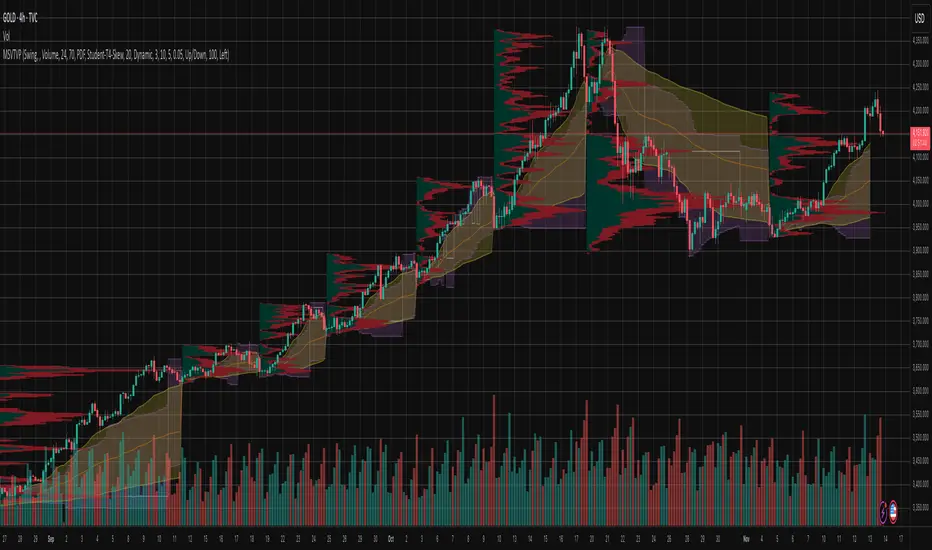
Market Structure Volume Time Velocity ProfileThis is the Market Structure Volume Time Velocity Profile (MSVTVP). It combines event-based profiling with advanced metrics like Time and Velocity (Flow Rate). Instead of fixed time periods, profiles are anchored to critical market events (Swings, Structure Breaks, Delta Breaks), giving you a precise view of value development during specific market phases.
## The 3 Dimensions of the Market
Unlike standard tools that only show Volume, MSVTVP allows you
to switch between three critical metrics:
1. **VOLUME Profile (The "Where"):**
* Shows standard acceptance. High volume nodes (HVN)
are magnets for price.
2. **TIME Profile (The "How Long"):**
* Similar to TPO, it measures how long price spent at each
level.
* **High Time:** True acceptance and fair value.
* **Low Time:** Rejection or rapid movement.
3. **VELOCITY Profile (The "How Fast"):**
* Measures the **speed of trading** (Contracts per Second).
This reveals the hidden intent of market participants.
* **High Velocity (Fast Flow):** Aggression. Initiative
buyers/sellers are hitting market orders rapidly. Often
seen at breakouts or in liquidity vacu.
* **Low Velocity (Slow Flow):** Absorption. Massive passive
limit orders are slowing price down despite high volume.
Often seen at major reversals ("hitting a brick wall").
Key Features:
1. **Event-Based Profile Anchoring:** The indicator starts a new
profile based on one of three user-selected events
('Profile Anchor'):
- **Swing:** A new profile begins when the 'impulse baseline'
(derived from intra-bar delta) changes. This baseline
adjusts when a new **price pivot** is confirmed: When a
price **high** forms, the baseline moves to the **lower**
of its previous level or the peak delta (max of
delta O/C) at the pivot. When a price **low** forms, it
moves to the **higher** of its previous level or the
trough delta (min of delta O/C) at the pivot.
- **Structure:** A new profile begins immediately on the bar
that *confirms* a market structure break (e.g., a new HH
or LL, based on a sequence of price pivots).
- **Delta:** A new profile begins immediately on the bar
that *confirms* a break in the *cumulative delta's*
market structure (e.g., a new HH or LL in the delta).
Both 'Swing' and 'Delta' anchors are derived from the same
**continuous (non-resetting) Cumulative Volume Profile Delta (CVPD)**,
which is built from the intra-bar statistical analysis.
2. **Statistical Profile Engine:** For each bar in the anchored
period, the indicator builds a volume profile on a lower
'Intra-Bar Timeframe'. Instead of simple tick counting, it
uses advanced statistical models:
- **Allocation ('Allot model'):** 'PDF' (Probability Density
Function) distributes volume proportionally across the
bar's range based on an assumed statistical model
(e.g., T4-Skew). 'Classic' assigns all volume to
the close.
- **Buy/Sell Split ('Volume Estimator'):** 'Dynamic'
applies a model that analyzes candle wicks and
recent trend to estimate buy/sell pressure. 'Classic'
classifies all volume based on the candle color.
3. **Visualization & Lag:** The indicator plots the final
profile (as a polygon) and the developing statistical
lines (POC, VA, VWAP, StdDev).
- **Note on Lag:** All anchor events require `Pivot Right Bars`
for confirmation.
- In 'Structure' and 'Delta' mode, the developing lines
(POC, VA, etc.) are plotted using a **non-repainting**
method (showing the value from `pivRi` bars ago).
- In 'Swing' mode, the profile is plotted **retroactively**,
starting *from the bar where the pivot occurred*. The
developing lines are also plotted with this full
`pivRi` lag to align with the past data.
4. **Flexible Display Modes:** The finalized profile can be displayed
in three ways: 'Up/Down' (buy vs. sell), 'Total' (combined
volume), and 'Delta' (net difference).
5. **Dynamic Row Sizing:** Includes an option ('Rows per Percent')
to automatically adjust the number of profile rows (buckets)
based on the profile's price range.
6. **Integrated Alerts:** Includes 13 alerts that trigger for:
- A new profile reset ('Profile was resetted').
- Price crossing any of the 6 developing levels (POC,
VA High/Low, VWAP, StdDev High/Low).
- **Alert Lag Assumption:** In 'Swing' mode, alerts are
delayed to match the retroactively plotted lines.
In 'Structure' and 'Delta' modes, alerts fire in
**real-time** based on the *current price* crossing
the *current (repainting)* value of the metric, which
may **differ from the non-repainting plotted line.**
**Caution: Real-Time Data Behavior (Intra-Bar Repainting)**
This indicator uses high-resolution intra-bar data. As a result, the
values on the **current, unclosed bar** (the real-time bar) will
update dynamically as new intra-bar data arrives. This includes
the values used for real-time alerts in 'Structure' and
'Delta' modes.
---
**DISCLAIMER**
1. **For Informational/Educational Use Only:** This indicator is
provided for informational and educational purposes only. It does
not constitute financial, investment, or trading advice, nor is
it a recommendation to buy or sell any asset.
2. **Use at Your Own Risk:** All trading decisions you make based on
the information or signals generated by this indicator are made
solely at your own risk.
3. **No Guarantee of Performance:** Past performance is not an
indicator of future results. The author makes no guarantee
regarding the accuracy of the signals or future profitability.
4. **No Liability:** The author shall not be held liable for any
financial losses or damages incurred directly or indirectly from
the use of this indicator.
5. **Signals Are Not Recommendations:** The alerts and visual signals
(e.g., crossovers) generated by this tool are not direct
recommendations to buy or sell. They are technical observations
for your own analysis and consideration.
ابحث في النصوص البرمجية عن "poc"
LibVeloLibrary "LibVelo"
This library provides a sophisticated framework for **Velocity
Profile (Flow Rate)** analysis. It measures the physical
speed of trading at specific price levels by relating volume
to the time spent at those levels.
## Core Concept: Market Velocity
Unlike Volume Profiles, which only answer "how much" traded,
Velocity Profiles answer "how fast" it traded.
It is calculated as:
`Velocity = Volume / Duration`
This metric (contracts per second) reveals hidden market
dynamics invisible to pure Volume or TPO profiles:
1. **High Velocity (Fast Flow):**
* **Aggression:** Initiative buyers/sellers hitting market
orders rapidly.
* **Liquidity Vacuum:** Price slips through a level because
order book depth is thin (low resistance).
2. **Low Velocity (Slow Flow):**
* **Absorption:** High volume but very slow price movement.
Indicates massive passive limit orders ("Icebergs").
* **Apathy:** Little volume over a long time. Lack of
interest from major participants.
## Architecture: Triple-Engine Composition
To ensure maximum performance while offering full statistical
depth for all metrics, this library utilises **object
composition** with a lazy evaluation strategy:
#### Engine A: The Master (`vpVol`)
* **Role:** Standard Volume Profile.
* **Purpose:** Maintains the "ground truth" of volume distribution,
price buckets, and ranges.
#### Engine B: The Time Container (`vpTime`)
* **Role:** specialized container for time duration (in ms).
* **Hack:** It repurposes standard volume arrays (specifically
`aBuy`) to accumulate time duration for each bucket.
#### Engine C: The Calculator (`vpVelo`)
* **Role:** Temporary scratchpad for derived metrics.
* **Purpose:** When complex statistics (like Value Area or Skewness)
are requested for **Velocity**, this engine is assembled
on-demand to leverage the full statistical power of `LibVPrf`
without rewriting complex algorithms.
---
**DISCLAIMER**
This library is provided "AS IS" and for informational and
educational purposes only. It does not constitute financial,
investment, or trading advice.
The author assumes no liability for any errors, inaccuracies,
or omissions in the code. Using this library to build
trading indicators or strategies is entirely at your own risk.
As a developer using this library, you are solely responsible
for the rigorous testing, validation, and performance of any
scripts you create based on these functions. The author shall
not be held liable for any financial losses incurred directly
or indirectly from the use of this library or any scripts
derived from it.
create(buckets, rangeUp, rangeLo, dynamic, valueArea, allot, estimator, cdfSteps, split, trendLen)
Construct a new `Velo` controller, initializing its engines.
Parameters:
buckets (int) : series int Number of price buckets ≥ 1.
rangeUp (float) : series float Upper price bound (absolute).
rangeLo (float) : series float Lower price bound (absolute).
dynamic (bool) : series bool Flag for dynamic adaption of profile ranges.
valueArea (int) : series int Percentage for Value Area (1..100).
allot (series AllotMode) : series AllotMode Allocation mode `Classic` or `PDF` (default `PDF`).
estimator (series PriceEst enum from AustrianTradingMachine/LibBrSt/1) : series PriceEst PDF model for distribution attribution (default `Uniform`).
cdfSteps (int) : series int Resolution for PDF integration (default 20).
split (series SplitMode) : series SplitMode Buy/Sell split for the master volume engine (default `Classic`).
trendLen (int) : series int Look‑back for trend factor in dynamic split (default 3).
Returns: Velo Freshly initialised velocity profile.
method clone(self)
Create a deep copy of the composite profile.
Namespace types: Velo
Parameters:
self (Velo) : Velo Profile object to copy.
Returns: Velo A completely independent clone.
method clear(self)
Reset all engines and accumulators.
Namespace types: Velo
Parameters:
self (Velo) : Velo Profile object to clear.
Returns: Velo Cleared profile (chaining).
method merge(self, srcVolBuy, srcVolSell, srcTime, srcRangeUp, srcRangeLo, srcVolCvd, srcVolCvdHi, srcVolCvdLo)
Merges external data (Volume and Time) into the current profile.
Automatically handles resizing and re-bucketing if ranges differ.
Namespace types: Velo
Parameters:
self (Velo) : Velo The profile object.
srcVolBuy (array) : array Source Buy Volume bucket array.
srcVolSell (array) : array Source Sell Volume bucket array.
srcTime (array) : array Source Time bucket array (ms).
srcRangeUp (float) : series float Upper price bound of the source data.
srcRangeLo (float) : series float Lower price bound of the source data.
srcVolCvd (float) : series float Source Volume CVD final value.
srcVolCvdHi (float) : series float Source Volume CVD High watermark.
srcVolCvdLo (float) : series float Source Volume CVD Low watermark.
Returns: Velo `self` (chaining).
method addBar(self, offset)
Main data ingestion. Distributes Volume and Time to buckets.
Namespace types: Velo
Parameters:
self (Velo) : Velo The profile object.
offset (int) : series int Offset of the bar to add (default 0).
Returns: Velo `self` (chaining).
method setBuckets(self, buckets)
Sets the number of buckets for the profile.
Namespace types: Velo
Parameters:
self (Velo) : Velo The profile object.
buckets (int) : series int New number of buckets.
Returns: Velo `self` (chaining).
method setRanges(self, rangeUp, rangeLo)
Sets the price range for the profile.
Namespace types: Velo
Parameters:
self (Velo) : Velo The profile object.
rangeUp (float) : series float New upper price bound.
rangeLo (float) : series float New lower price bound.
Returns: Velo `self` (chaining).
method setValueArea(self, va)
Set the percentage of volume/time for the Value Area.
Namespace types: Velo
Parameters:
self (Velo) : Velo The profile object.
va (int) : series int New Value Area percentage (0..100).
Returns: Velo `self` (chaining).
method getBuckets(self)
Returns the current number of buckets in the profile.
Namespace types: Velo
Parameters:
self (Velo) : Velo The profile object.
Returns: series int The number of buckets.
method getRanges(self)
Returns the current price range of the profile.
Namespace types: Velo
Parameters:
self (Velo) : Velo The profile object.
Returns:
rangeUp series float The upper price bound of the profile.
rangeLo series float The lower price bound of the profile.
method getArrayBuyVol(self)
Returns the internal raw data array for **Buy Volume** directly.
Namespace types: Velo
Parameters:
self (Velo) : Velo The profile object.
Returns: array The internal array for buy volume.
method getArraySellVol(self)
Returns the internal raw data array for **Sell Volume** directly.
Namespace types: Velo
Parameters:
self (Velo) : Velo The profile object.
Returns: array The internal array for sell volume.
method getArrayTime(self)
Returns the internal raw data array for **Time** (in ms) directly.
Namespace types: Velo
Parameters:
self (Velo) : Velo The profile object.
Returns: array The internal array for time duration.
method getArrayBuyVelo(self)
Returns the internal raw data array for **Buy Velocity** directly.
Automatically executes _assemble() if data is dirty.
Namespace types: Velo
Parameters:
self (Velo) : Velo The profile object.
Returns: array The internal array for buy velocity.
method getArraySellVelo(self)
Returns the internal raw data array for **Sell Velocity** directly.
Automatically executes _assemble() if data is dirty.
Namespace types: Velo
Parameters:
self (Velo) : Velo The profile object.
Returns: array The internal array for sell velocity.
method getBucketBuyVol(self, idx)
Returns the **Buy Volume** of a specific bucket.
Namespace types: Velo
Parameters:
self (Velo) : Velo The profile object.
idx (int) : series int The index of the bucket.
Returns: series float The buy volume.
method getBucketSellVol(self, idx)
Returns the **Sell Volume** of a specific bucket.
Namespace types: Velo
Parameters:
self (Velo) : Velo The profile object.
idx (int) : series int The index of the bucket.
Returns: series float The sell volume.
method getBucketTime(self, idx)
Returns the raw accumulated time (in ms) spent in a specific bucket.
Namespace types: Velo
Parameters:
self (Velo) : Velo The profile object.
idx (int) : series int The index of the bucket.
Returns: series float The time in milliseconds.
method getBucketBuyVelo(self, idx)
Returns the **Buy Velocity** (Aggressive Buy Flow) of a bucket.
Namespace types: Velo
Parameters:
self (Velo) : Velo The profile object.
idx (int) : series int The index of the bucket.
Returns: series float The buy velocity in .
method getBucketSellVelo(self, idx)
Returns the **Sell Velocity** (Aggressive Sell Flow) of a bucket.
Namespace types: Velo
Parameters:
self (Velo) : Velo The profile object.
idx (int) : series int The index of the bucket.
Returns: series float The sell velocity in .
method getBktBnds(self, idx)
Returns the price boundaries of a specific bucket.
Namespace types: Velo
Parameters:
self (Velo) : Velo The profile object.
idx (int) : series int The index of the bucket.
Returns:
up series float The upper price bound of the bucket.
lo series float The lower price bound of the bucket.
method getPoc(self, target)
Returns Point of Control (POC) information for the specified target metric.
Calculates on-demand if the target is 'Velocity' and data changed.
Namespace types: Velo
Parameters:
self (Velo) : Velo The profile object.
target (series Metric) : Metric The data aspect to analyse (Volume, Time, Velocity).
Returns:
pocIdx series int The index of the POC bucket.
pocPrice series float The mid-price of the POC bucket.
method getVA(self, target)
Returns Value Area (VA) information for the specified target metric.
Calculates on-demand if the target is 'Velocity' and data changed.
Namespace types: Velo
Parameters:
self (Velo) : Velo The profile object.
target (series Metric) : Metric The data aspect to analyse (Volume, Time, Velocity).
Returns:
vaUpIdx series int The index of the upper VA bucket.
vaUpPrice series float The upper price bound of the VA.
vaLoIdx series int The index of the lower VA bucket.
vaLoPrice series float The lower price bound of the VA.
method getMedian(self, target)
Returns the Median price for the specified target metric distribution.
Calculates on-demand if the target is 'Velocity' and data changed.
Namespace types: Velo
Parameters:
self (Velo) : Velo The profile object.
target (series Metric) : Metric The data aspect to analyse (Volume, Time, Velocity).
Returns:
medianIdx series int The index of the bucket containing the median.
medianPrice series float The median price.
method getAverage(self, target)
Returns the weighted average price (VWAP/TWAP) for the specified target.
Calculates on-demand if the target is 'Velocity' and data changed.
Namespace types: Velo
Parameters:
self (Velo) : Velo The profile object.
target (series Metric) : Metric The data aspect to analyse (Volume, Time, Velocity).
Returns:
avgIdx series int The index of the bucket containing the average.
avgPrice series float The weighted average price.
method getStdDev(self, target)
Returns the standard deviation for the specified target distribution.
Calculates on-demand if the target is 'Velocity' and data changed.
Namespace types: Velo
Parameters:
self (Velo) : Velo The profile object.
target (series Metric) : Metric The data aspect to analyse (Volume, Time, Velocity).
Returns: series float The standard deviation.
method getSkewness(self, target)
Returns the skewness for the specified target distribution.
Calculates on-demand if the target is 'Velocity' and data changed.
Namespace types: Velo
Parameters:
self (Velo) : Velo The profile object.
target (series Metric) : Metric The data aspect to analyse (Volume, Time, Velocity).
Returns: series float The skewness.
method getKurtosis(self, target)
Returns the excess kurtosis for the specified target distribution.
Calculates on-demand if the target is 'Velocity' and data changed.
Namespace types: Velo
Parameters:
self (Velo) : Velo The profile object.
target (series Metric) : Metric The data aspect to analyse (Volume, Time, Velocity).
Returns: series float The excess kurtosis.
method getSegments(self, target)
Returns the fundamental unimodal segments for the specified target metric.
Calculates on-demand if the target is 'Velocity' and data changed.
Namespace types: Velo
Parameters:
self (Velo) : Velo The profile object.
target (series Metric) : Metric The data aspect to analyse (Volume, Time, Velocity).
Returns: matrix A 2-column matrix where each row is an pair.
method getCvd(self, target)
Returns Cumulative Volume/Velo Delta (CVD) information for the target metric.
Namespace types: Velo
Parameters:
self (Velo) : Velo The profile object.
target (series Metric) : Metric The data aspect to analyse (Volume, Time, Velocity).
Returns:
cvd series float The final delta value.
cvdHi series float The historical high-water mark of the delta.
cvdLo series float The historical low-water mark of the delta.
Velo
Velo Composite Velocity Profile Controller.
Fields:
_vpVol (VPrf type from AustrianTradingMachine/LibVPrf/2) : LibVPrf.VPrf Engine A: Master Volume source.
_vpTime (VPrf type from AustrianTradingMachine/LibVPrf/2) : LibVPrf.VPrf Engine B: Time duration container (ms).
_vpVelo (VPrf type from AustrianTradingMachine/LibVPrf/2) : LibVPrf.VPrf Engine C: Scratchpad for velocity stats.
_aTime (array) : array Pointer alias to `vpTime.aBuy` (Time storage).
_valueArea (series float) : int Percentage of total volume to include in the Value Area (1..100)
_estimator (series PriceEst enum from AustrianTradingMachine/LibBrSt/1) : LibBrSt.PriceEst PDF model for distribution attribution.
_allot (series AllotMode) : AllotMode Attribution model (Classic or PDF).
_cdfSteps (series int) : int Integration resolution for PDF.
_isDirty (series bool) : bool Lazy evaluation flag for vpVelo.

RBD Market ProfileA Market Profile visually shows how much time (or how many bars) price spent at each price level within a session — helping identify areas of “fair value” (where price spent most time) and extremes (where price barely traded).
It divides each trading session (for example, a day, week, or month depending on input) into price segments, counts how many bars closed within each segment, and then identifies:
POC (Point of Control): price level with the highest frequency (most traded or visited).
VAH (Value Area High): upper boundary of the zone that contains 70% (or user-defined percentage) of all activity around the POC.
VAL (Value Area Low): lower boundary of that same 70% activity zone.
Finally, it plots lines for:
VAH (green line)
VAL (red line)
POC Upper & Lower (white lines)
Session Open (blue dashed line)
How to use this Market Profile:
Determine Key Areas of Support/Resistance by the VAH and VAL
VAH: Responsive Sellers and Initiative Buyers
VAL: Responsive Buyers and Initiative Sellers
POC: Can be used as Fair Value

Market Structure Volume ProfileThis indicator visualizes volume profiles that are dynamically anchored to market structure events, rather than fixed time intervals. It builds these profiles using high-resolution intra-bar data to provide a precise view of where value is established during critical market phases.
Key Features:
Event-Based Profile Anchoring: The indicator starts a new profile based on one of three user-selected events ('Profile Anchor'):
Swing: A new profile begins when the 'impulse baseline' (derived from intra-bar delta) changes. This baseline adjusts when a new price pivot is confirmed: When a price high forms, the baseline moves to the lower of its previous level or the peak delta (max of delta O/C) at the pivot. When a price low forms, it moves to the higher of its previous level or the trough delta (min of delta O/C) at the pivot.
Structure: A new profile begins immediately on the bar that confirms a market structure break (e.g., a new HH or LL, based on a sequence of price pivots).
Delta: A new profile begins immediately on the bar that confirms a break in the cumulative delta's market structure (e.g., a new HH or LL in the delta). Both 'Swing' and 'Delta' anchors are derived from the same continuous (non-resetting) Cumulative Volume Profile Delta (CVPD), which is built from the intra-bar statistical analysis.
Statistical Profile Engine: For each bar in the anchored period, the indicator builds a volume profile on a lower 'Intra-Bar Timeframe'. Instead of simple tick counting, it uses advanced statistical models:
Allocation ('Allot model'): 'PDF' (Probability Density Function) distributes volume proportionally across the bar's range based on an assumed statistical model (e.g., T4-Skew). 'Classic' assigns all volume to the close.
Buy/Sell Split ('Volume Estimator'): 'Dynamic' applies a model that analyzes candle wicks and recent trend to estimate buy/sell pressure. 'Classic' classifies all volume based on the candle color.
Visualization & Lag: The indicator plots the final profile (as a polygon) and the developing statistical lines (POC, VA, VWAP, StdDev).
Note on Lag: All anchor events require Pivot Right Bars for confirmation.
In 'Structure' and 'Delta' mode, the developing lines (POC, VA, etc.) are plotted using a non-repainting method (showing the value from pivRi bars ago).
In 'Swing' mode, the profile is plotted retroactively, starting from the bar where the pivot occurred. The developing lines are also plotted with this full pivRi lag to align with the past data.
Flexible Display Modes: The finalized profile can be displayed in three ways: 'Up/Down' (buy vs. sell), 'Total' (combined volume), and 'Delta' (net difference).
Dynamic Row Sizing: Includes an option ('Rows per Percent') to automatically adjust the number of profile rows (buckets) based on the profile's price range.
Integrated Alerts: Includes 13 alerts that trigger for:
A new profile reset ('Profile was resetted').
Price crossing any of the 6 developing levels (POC, VA High/Low, VWAP, StdDev High/Low).
Alert Lag Assumption: In 'Swing' mode, alerts are delayed to match the retroactively plotted lines. In 'Structure' and 'Delta' modes, alerts fire in real-time based on the current price crossing the current (repainting) value of the metric, which may differ from the non-repainting plotted line.
Caution: Real-Time Data Behavior (Intra-Bar Repainting) This indicator uses high-resolution intra-bar data. As a result, the values on the current, unclosed bar (the real-time bar) will update dynamically as new intra-bar data arrives. This includes the values used for real-time alerts in 'Structure' and 'Delta' modes.
DISCLAIMER
For Informational/Educational Use Only: This indicator is provided for informational and educational purposes only. It does not constitute financial, investment, or trading advice, nor is it a recommendation to buy or sell any asset.
Use at Your Own Risk: All trading decisions you make based on the information or signals generated by this indicator are made solely at your own risk.
No Guarantee of Performance: Past performance is not an indicator of future results. The author makes no guarantee regarding the accuracy of the signals or future profitability.
No Liability: The author shall not be held liable for any financial losses or damages incurred directly or indirectly from the use of this indicator.
Signals Are Not Recommendations: The alerts and visual signals (e.g., crossovers) generated by this tool are not direct recommendations to buy or sell. They are technical observations for your own analysis and consideration.

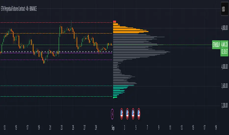
Extreme Zone Volume ProfileExtreme Zone Volume Profile (EZVP)
Originality & Innovation
The Extreme Zone Volume Profile (EZVP) revolutionizes traditional volume profile analysis by applying statistical zone classification to volume distribution. Unlike standard volume profiles that display raw volume data, EZVP segments the price range into statistically meaningful zones based on percentile thresholds, allowing traders to instantly identify where volume concentration suggests strong support/resistance versus areas of potential breakout.
Technical Methodology
Core Algorithm:
Distributes volume across user-defined bins (20-200) over a lookback period
Calculates volume-weighted price levels for each bin
Applies percentile-based zone classification to the price range (not volume ranking)
Zone B (extreme zones): Outer percentile tails representing potential rejection areas
Zone A (significant zones): Secondary percentile bands indicating strong interest levels
Center Zone: Bulk trading range where most price discovery occurs
Mathematical Foundation:
The script uses price-range percentiles rather than volume percentiles. If the total price range is divided into 100%, Zone B captures the extreme price tails (default 2.5% each end ≈ 2 standard deviations), Zone A captures the next significant bands (default 14% each ≈ 1 standard deviation), leaving the center for normal distribution trading.
Key Calculations:
POC (Point of Control): Price level with maximum volume accumulation
Volume-weighted mean price: Total volume × price / total volume
Median price: Geometric center of the price range
Rightward-projected bars: Volume bars extend forward from current time to avoid historical chart clutter
Trading Applications
Zone Interpretation:
Zone B (Red/Green): Extreme price levels where volume suggests strong rejection potential. Price reaching these zones often indicates overextension and possible reversal points.
Zone A (Orange/Teal): Significant support/resistance areas with substantial volume interest. These levels often act as intermediate targets or consolidation zones.
Center (Gray): Fair value area where most trading occurs. Price tends to return to this range during normal market conditions.
Strategic Usage:
Reversal Trading: Look for rejection signals when price enters Zone B areas
Breakout Confirmation: Volume expansion beyond Zone B boundaries suggests genuine breakouts
Support/Resistance: Zone A boundaries often provide reliable entry/exit levels
Mean Reversion: Price tends to gravitate toward the volume-weighted mean and POC lines
Unique Value Proposition
EZVP addresses three key limitations of traditional volume profiles:
Visual Clarity: Standard profiles can be cluttered and difficult to interpret quickly. EZVP's color-coded zones provide instant visual feedback about price significance.
Statistical Framework: Rather than relying on subjective interpretation of volume nodes, EZVP applies objective percentile-based classification, making support/resistance identification more systematic.
Forward-Looking Display: Rightward-projecting bars keep historical price action clean while maintaining current market structure visibility.
Configuration Guide
Lookback Period (10-1000): Controls the historical depth of volume calculation. Shorter periods for intraday scalping, longer for swing trading.
Number of Bins (20-200): Resolution of volume distribution. Higher values provide more granular analysis but may create noise on lower timeframes.
Zone Percentages:
Zone B: Extreme threshold (default 2.5% = ~2σ statistical significance)
Zone A: Significant threshold (default 14% = ~1σ statistical significance)
Visual Controls: Toggle individual elements (POC, median, mean, zone lines) to customize display complexity for your trading style.
Technical Requirements
Pine Script v6 compatible
Maximum bars back: 5000 (ensures sufficient historical data)
Maximum boxes: 500 (supports high-resolution bin counts)
Maximum lines: 50 (accommodates all zone and reference lines)
This indicator synthesizes volume profile theory with statistical zone analysis, providing a quantitative framework for identifying high-probability support/resistance levels based on volume distribution patterns rather than arbitrary price levels.
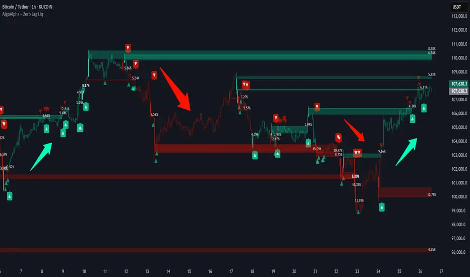
Zero Lag Liquidity [AlgoAlpha]🟠 OVERVIEW
This script plots liquidity zones with zero lag using lower-timeframe wick profiles and high-volume wicks to mark key price reactions. It’s called Zero Lag Liquidity because it captures significant liquidity imbalances in real time by processing lower-TF price-volume distributions directly inside the wick of abnormal candles. The tool builds a volume histogram inside long upper/lower wicks, then calculates a local Point of Control (POC) to mark the price where most volume occurred. These levels act as visual liquidity zones, which can trigger labels, break signals, and trend detection depending on price interaction.
🟠 CONCEPTS
The core concept relies on identifying high-volume candles with unusually long wicks—often a sign of opposing liquidity. When a large upper or lower wick appears with a strong volume spike, the script builds a histogram of lower-timeframe closes and volumes inside that wick. It bins the wick into segments, sums volume per bin, and finds the POC. This POC becomes the liquidity level. The script then dynamically tracks whether price breaks above or rejects off these levels, adjusts the active trend regime accordingly, and highlights bars to help users spot continuation or reversal behavior. The logic avoids repainting or subjective interpretation by using fixed thresholds and lower-TF price action.
🟠 FEATURES
Dynamic liquidity levels rendered at POC of significant wicks, colored by bullish/bearish direction.
Break detection that removes levels once price decisively crosses them twice in the same direction.
Rejection detection that plots ▲/▼ markers when price bounces off levels intrabar.
Volume labels for each level, shown either as raw volume or percentage of total level volume.
Candle coloring based on trend direction (break-dominant).
🟠 USAGE
Use this indicator to track where liquidity has most likely entered the market via abnormal wick events. When a long wick forms with high volume, the script looks inside it (using your chosen lower timeframe) and marks the most traded price within it. These levels can serve as expected reversal or breakout zones. Rejections are marked with small arrows, while breaks trigger trend shifts and remove the level. You can toggle trend coloring to see directional bias after a breakout. Use the wick multiplier to control how selective the detector is (higher = stricter). Alerts and label modes help customize the signal for different asset types and chart styles.
Overnight Bias: Net Long/Short with PercentOvernight bias can assist with NY session gap fades or gap and go trading once the NY session is open.
Some general gap rules are:
1. Gap Direction Aligned with Overnight Bias
Rule: If the NY session gaps up and the overnight bias is Net Long (e.g., >60% of bars above the overnight open), favor longs.
Confirmation: Look for price to hold above overnight open or VWAP.
Invalidation: If price re-enters the overnight range, reassess.
2. Gap Opposing Overnight Bias (Contrarian Setup)
Rule: If the NY opens opposite the overnight bias, expect potential gap fill or reversal.
Trade Bias: Look for retracement back toward the overnight open or VWAP.
Example: Overnight was Net Long, but NY gaps down → wait for reclaim of VWAP to go long, else fade strength.
3. Gap Into Prior Day Value Area (VAH to VAL)
Rule: If the NY session gaps into the prior day value area:
It implies mean reversion behavior.
Expect price to rotate toward the POC (point of control).
Trade Bias: Fade toward POC if overnight bias is balanced or opposite the gap direction.
4. Gap Outside Prior Day Value Area
Rule: A gap above VAH or below VAL suggests potential breakout or new trend day.
Trade Bias: If overnight bias aligns (e.g., gap above VAH + Net Long overnight), consider trend continuation.
Invalidation: If price breaks back inside the prior day value area, watch for failed breakout → fade trade possible.
5. Gap Above Prior Day High / Below Prior Day Low
Rule: This is a true breakout gap.
Above Prior High + Net Long Bias: Look for continuation.
Below Prior Low + Net Short Bias: Look for sell pressure continuation.
Trade Bias: Use pullbacks to the prior high/low or overnight open for continuation setups.
6. Gap Within Prior Day Range
Rule: If the NY open is within the prior day’s high and low, expect chop or balanced conditions.
Trade Bias: Use overnight VWAP and prior POC as decision zones. Be cautious unless a breakout occurs.
7. Failed Gap and Re-entry into Prior Day Range
Rule: If price gaps above prior high but re-enters the prior range, it's a failed breakout.
Trade Bias: Look for a fade back to VAH or POC.
Confirmation: Watch for breakdown below overnight VWAP or failure to hold overnight open.
8. Gap + Overnight VWAP Divergence
Rule: If price gaps opposite the direction of VWAP (e.g., VWAP rising, gap down), wait for confirmation.
Trade Bias: Be cautious with early trades. Bias may flip if VWAP is reclaimed.
9. Gap + Overnight Open Test
Rule: If price opens with a gap and then retests the overnight open, that level becomes a decision zone.
Trade Bias:
Hold above = trend continuation.
Rejection = gap fill or reversal.
10. Unfilled Gap = Trend Bias
Rule: If the gap remains unfilled for the first 30–60 minutes, it increases the odds of a trend day.
Trade Bias: Trade pullbacks in the direction of the gap and overnight bias.
Should anyone have suggestion to add please do so.

volume profile ranking indicator📌 Introduction
This script implements a volume profile ranking indicato for TradingView. It is designed to visualize the distribution of traded volume over price levels within a defined historical window. Unlike TradingView’s built-in Volume Profile, this script gives full customization of the profile drawing logic, binning, color gradient, and the ability to anchor the profile to a specific date.
⚙️ How It Works (Logic)
1. Inputs
➤POC Lookback Days (lookback): Defines how many bars (days) to look back from a selected point to calculate the volume distribution.
➤Bin Count (bin_count): Determines how many price bins (horizontal levels) the price range will be divided into.
➤Use Custom Lookback Date (useCustomDate): Enables/disables manually selecting a backtest start date.
➤Custom Lookback Date (customDate): When enabled, the profile will calculate volume based on this date instead of the most recent bar.
2. Target Bar Determination
➤If a custom date is selected, the script searches for the bar closest to that date within 1000 bars.
➤If not, it defaults to the latest bar (bar_index).
➤The profile is drawn only when the current bar is close to the target bar (within ±2 bars), to avoid unnecessary recalculations and performance issues.
3. Volume Binning
➤The price range over the lookback window is divided into bin_count segments.
➤For each bar within the lookback window, its volume is added to the appropriate bin based on price.
➤If the price falls outside the expected range, it is clamped to the first or last bin.
4. Ranking and Sorting
➤A bubble sort ranks each bin by total volume.
➤The most active bin (POC, or Point of Control) is highlighted with a thicker bar.
5. Rendering
➤Horizontal bars (line.new) represent volume intensity in each price bin.
➤Each bar is color-coded by volume heat: more volume = more intense color.
➤Labels (label.new) show:
➤Total volume
➤Rank
➤Percentage of total volume
➤Price range of the bin
🧑💻 How to Use
1. Add the Script to Your Chart
➤Copy the code into TradingView’s Pine Script editor and add it to your chart.
2. Set Lookback Period
➤Default is 252 bars (about one year for daily charts), but can be changed via the input.
3. (Optional) Use Custom Date
●Toggle "Use Custom Lookback Date" to true.
➤Pick a date in the "Custom Lookback Date" input to anchor the profile.
4. Analyze the Volume Distribution
➤The longest (thickest) red/orange bar represents the Point of Control (POC) — the price with the most volume traded.
➤Other bars show volume distribution across price.
➤Labels display useful metrics to evaluate areas of high/low interest.
✅ Features
🔶 Customizable anchor point (custom date).
🔶Adjustable bin count and lookback length.
🔶 Clear visualization with heatmap coloring.
🔶 Lightweight and performance-optimized (especially with the shouldDrawProfile filter)

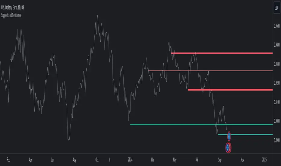
Support and ResistanceThis indicator, titled "Support and Resistance," is designed to identify and display key price levels based on volume and pivot points. It's a versatile tool that can be adapted for different market views and timeframes.
Key Features
Market View Options
The indicator offers three market view settings:
Short term
Standard
Long term
These settings affect the lookback periods used in calculations, allowing users to adjust the indicator's sensitivity to market movements.
Volume-Based Levels
The indicator calculates support and resistance levels using a rolling Point of Control (POC) derived from volume data. This approach helps identify price levels where the most trading activity has occurred.
Pivot Points
In addition to volume-based levels, the indicator incorporates pivot points to identify potential support and resistance areas.
Customizable Appearance
Users can adjust:
Number of lines to display (1-8)
Colors for support and resistance levels
Line thickness based on level importance
Calculation Methods
Rolling POC
The indicator uses a custom function f_rolling_poc to calculate the rolling Point of Control. This function analyzes volume distribution across price levels within a specified lookback period.
Pivot Points
Both standard and quick pivot points are calculated using the rolling POC as input, rather than traditional price data.
Level Importance
The indicator assigns importance to each level based on:
Number of touches (how often price has interacted with the level)
Duration (how long the level has been relevant)
This importance score determines the thickness of the displayed lines.
Unique Aspects
Dynamic Line Thickness: Lines become thicker when levels overlap, highlighting potentially stronger support/resistance areas.
Adaptive Coloring: The color of each line changes dynamically based on whether the current price is above or below the level, indicating whether it's acting as support or resistance.
Flexible Time Frames: The market view options allow the indicator to be easily adapted for different trading styles and timeframes.
Potential Uses
This indicator could be valuable for:
Identifying key price levels for entry and exit points
Recognizing potential breakout or breakdown levels
Understanding the strength of support and resistance based on line thickness
Adapting analysis to different market conditions and timeframes
Overall, this "Support and Resistance" indicator offers a sophisticated approach to identifying key price levels, combining volume analysis with pivot points and providing visual cues for level importance and current market position.
This Support and Resistance indicator is provided for informational and educational purposes only. It should not be considered as financial advice or a recommendation to buy or sell any security. The indicator's calculations are based on historical data and may not accurately predict future market movements. Trading decisions should be made after thorough research and consultation with a licensed financial advisor. The creator of this indicator is not responsible for any losses incurred from its use. Past performance does not guarantee future results. Use at your own risk.
Depth of Market (DOM) [LuxAlgo]The Depth Of Market (DOM) tool allows traders to look under the hood of any market, taking price and volume analysis to the next level. The following features are included: DOM, Time & Sales, Volume Profile, Depth of Market, Imbalances, Buying Pressure, and up to 24 key intraday levels (it really packs a punch).
As a disclaimer, this tool does not use tick data, it is a DOM reconstruction from the provided real-time time series data (price and volume). So the volume you see is from filled orders only, this tool does not show unfilled limit orders.
Traders can enable or disable any of the features at will to avoid being overwhelmed with too much information and to make the tool perform faster.
The features that have the biggest impact on performance are Historical Data Collection, Key Levels (POC & VWAP), Time & Sales, Profile, and Imbalances. Disable these features to improve the indicator computational performance.
🔶 DOM
This is the simplest form of the tool, a simple DOM or ladder that displays the following columns:
PRICE: Price level
BID: Total number of market sell orders filled or limit buy orders filled.
SELL: Sell market orders
BUY: Buy market orders
ASK: Total number of market buy orders filled or limit sell orders filled.
The DOM only collects historical data from the last 24 hours and real-time data.
Traders can select a reset period for the DOM with two options:
DAILY: Resets at the beginning of each trading day
SESSIONS: Resets twice, as DAILY and 15.5 hours later, to coincide with the start of the RTH session for US tickers.
The DOM has two main modes, it can display price levels as ticks or points. The default is automatic based on the current daily volatility, but traders can manually force one mode or the other if they wish.
For convenience, traders have the option to set the number of lines (price levels), and the size of the text and to display only real-time data.
By default, the top price is set to 0 so that the DOM automatically adjusts the price levels to be displayed, but traders can set the top price manually so that the tool displays only the desired price levels in a fixed manner.
🔹 Volume Profile
As additional features to the basic DOM, traders have access to the volume profile histogram and the total volume per price level.
This helps traders identify at a glance key price areas where volume is accumulating (high volume nodes) or areas where volume is lacking (low volume nodes) - these areas are important to some traders who base their decision-making process on them.
🔹 Imbalances
Other added features are imbalances and buying pressure:
Interlevel Imbalance: volume delta between two different price levels
Intralevel Imbalance: delta between buy and sell volume at the same price level
Buying Pressure Percent: percentage of buy volume compared to total volume
Imbalances can help traders identify areas of interest in the price for possible support or resistance.
🔹 Depth
Depth allows traders to see at a glance how much supply is above the current price level or how much demand is below the current price level.
Above the current price level shows the cumulative ask volume (filled sell limit orders) and below the current price level shows the cumulative bid volume (filled buy limit orders).
🔶 KEY LEVELS
The tool includes up to 24 different key intraday levels of particular relevance:
Previous Week Levels
PWH: Previous week high
PWL: Previous week low
PWM: Previous week middle
PWS: Previous week settlement (close)
Previous Day Levels
PDH: Previous day high
PDL: Previous day low
PDM: Previous day middle
PDS: Previous day settlement (close)
Current Day Levels
OPEN: Open of day (or session)
HOD: High of day (or session)
LOD: Low of day (or session)
MOD: Middle of day (or session)
Opening Range
ORH: Open range high
ORL: Open range low
Initial Balance
IBH: Initial balance high
IBL: Initial balance low
VWAP
+3SD: Volume weighted average price plus 3 standard deviations
+2SD: Volume weighted average price plus 2 standard deviations
+1SD: Volume weighted average price plus 1 standard deviation
VWAP: Volume weighted average price
-1SD: Volume weighted average price minus 1 standard deviation
-2SD: Volume weighted average price minus 2 standard deviations
-3SD: Volume weighted average price minus 3 standard deviations
POC: Point of control
Different traders look at different levels, the key levels shown here are objective and specific areas of interest that traders can act on, providing us with potential areas of support or resistance in the price.
🔶 TIME & SALES
The tool also features a full-time and sales panel with time, price, and size columns, a size filter, and the ability to set the timezone to display time in the trader's local time.
The information shown here is what feeds the DOM and it can be useful in several ways, for example in detecting absorption. If a large number of orders are coming into the market but the price is barely moving, this indicates that there is enough liquidity at these levels to absorb all these orders, so if these orders stop coming into the market, the price may turn around.
🔶 SETTINGS
Period: Select the anchoring period to start data collection, DAILY will anchor at the start of the trading day, and SESSIONS will start as DAILY and 15.5 hours later (RTH for US tickers).
Mode: Select between AUTO and MANUAL modes for displaying TICKS or POINTS, in AUTO mode the tool will automatically select TICKS for tickers with a daily average volatility below 5000 ticks and POINTS for the rest of the tickers.
Rows: Select the number of price levels to display
Text Size: Select the text size
🔹 DOM
DOM: Enable/Disable DOM display
Realtime only: Enable/Disable real-time data only, historical data will be collected if disabled
Top Price: Specify the price to be displayed on the top row, set to 0 to enable dynamic DOM
Max updates: Specify how many times the values on the SELL and BUY columns are accumulated until reset.
Profile/Depth size: Maximum size of the histograms on the PROFILE and DEPTH columns.
Profile: Enable/Disable Profile column. High impact on performance.
Volume: Enable/Disable Volume column. Total volume traded at price level.
Interlevel Imbalance: Enable/Disable Interlevel Imbalance column. Total volume delta between the current price level and the price level above. High impact on performance.
Depth: Enable/Disable Depth, showing the cumulative supply above the current price and the cumulative demand below. Impact on performance.
Intralevel Imbalance: Enable/Disable Intralevel Imbalance column. Delta between total buy volume and total sell volume. High impact on performance.
Buying Pressure Percent: Enable/Disable Buy Percent column. Percentage of total buy volume compared to total volume.
Imbalance Threshold %: Threshold for highlighting imbalances. Set to 90 to highlight the top 10% of interlevel imbalances and the top and bottom 10% of intra-level imbalances.
Crypto volume precision: Specify the number of decimals to display on the volume of crypto assets
🔹 Key Levels
Key Levels: Enable/Disable KEY column. Very high performance impact.
Previous Week: Enable/Disable High, Low, Middle, and Close of the previous trading week.
Previous Day: Enable/Disable High, Low, Middle, and Settlement of the previous trading day.
Current Day/Session: Enable/Disable Open, High, Low and Middle of the current period.
Open Range: Enable/Disable High and Low of the first candle of the period.
Initial Balance: Enable/Disable High and Low of the first hour of the period.
VWAP: Enable/Disable Volume-weighted average price of the period with 1, 2, and 3 standard deviations.
POC: Enable/Disable Point of Control (price level with the highest volume traded) of the period.
🔹 Time & Sales
Time & Sales: Enable/Disable time and sales panel.
Timezone offset (hours): Enter your time zone\'s offset (+ or −), including a decimal fraction if needed.
Order Size: Set order size filter. Orders smaller than the value are not displayed.
🔶 THANKS
Hi, I'm makit0 coder of this tool and proud member of the LuxAlgo Opensource team, it's an honor to be part of the LuxAlgo family doing something I love as it's writing opensource code and sharing it with the world. I'd like to thank all of you who use, comment on, and vote for all of our open-source tools, and all of you who give us your support.
And of course thanks to the PineCoders family for all the work in front of and behind the scenes that makes the PineScript community what it is, simply the best.
Peace, Love & PineScript!

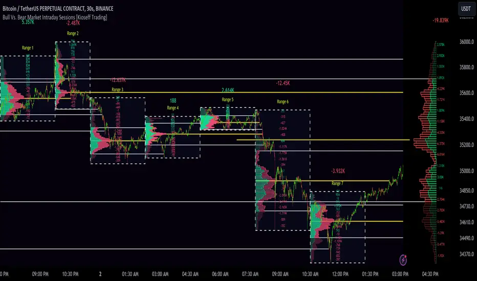
10x Bull Vs. Bear VP Intraday Sessions [Kioseff Trading]Hello!
This script "10x Bull Vs. Bear VP Intraday Sessions" lets the user configure up to 10 session ranges for Bull Vs. Bear volume profiles!
Features
Up To 10 Fixed Ranges!
Volume Profile Anchored to Fixed Range
Delta Ladder Anchored to Range
Bull vs Bear Profiles!
Standard Poc and Value Area Lines, in Addition to Separated POCs and Value Area Lines for Bull Profiles and Bear Profiles
Configurable Value Area Target
Up to 2000 Profile Rows per Visible Range
Stylistic Options for Profiles
This script generates Bull vs. Bear volume profiles for up to 10 fixed ranges!
Up to 2000 volume profile levels (price levels) Can be calculated for each profile, thanks to the new polyline feature, allowing for less aggregation / more precision of volume at price and volume delta.
Bull vs Bear Profiles
The image above shows primary functionality!
Green profiles = buying volume
Red profiles = selling volume
All colors are configurable.
Bullish & bearish POC + value areas for each fixed range are displayable!
That’s about it :D
This indicator is part of a series titled “Bull vs. Bear”.
If you have any suggestions please feel free to share!
OI Visible Range Ladder [Kioseff Trading]Hello!
This Script “OI Visible Range Ladder” calculates open interest profiles for the visible range alongside an OI ladder for the visible period!
Features
OI Profile Anchored to Visible Range
OI Ladder Anchored to Visible Range
Standard POC and Value Area Lines, in Addition to Separated POCs and Value Area Lines for each category of OI x Price
Configurable Value Area Targets
Curved Profiles
Up to 9999 Profile Rows per Visible Range
Stylistic Options for Profiles
Up to 9999 volume profile levels (Price levels) can be calculated for each profile, thanks to the new polyline feature, allowing for less aggregation / more precision of open interest at price.
The image above shows primary functionality!
Green profiles = Up OI / Up Price
Yellow profiles = Down OI / Up Price
Purple profiles = Up OI / Down Price
Red profiles = Down OI / Down Price
The image above shows POCs for each OI x Price category!
Profiles can be anchored on the left side for a more traditional look.
The indicator is robust enough to calculate on “small price periods”, or for a price period spanning your entire chart fully zoomed out!
That’s about it :D
This indicator is Part of a series titled “Bull vs. Bear” - a suite of profile-like indicators.
Thanks for checking this out!
If you have any suggestions please feel free to share!

Bull Vs Bear Visible Range VP [Kioseff Trading]Hello!
This Script “Bull vs Bear Visible Range VP” Calculates Bull & Bear Volume Profiles for the Visible Range Alongside a Delta Ladder for the Visible Period!
Features
Volume Profile Anchored to Visible Range
Delta Ladder Anchored to Visible Range
Bull vs Bear Profiles!
Standard Poc and Value Area Lines, in Addition to Separated POCs and Value Area Lines for Bull Profiles and Bear Profiles
Configurable Value Area Target
Curved Profiles
Up to 9999 Profile Rows per Visible Range
Stylistic Options for Profiles
This Script Generates Bull vs. Bear Volume Profiles for the Visible Range!
Up to 9999 Volume Profile Levels (Price Levels) Can Be Calculated for Each Profile, Thanks to the New Polyline Feature, Allowing For Less Aggregation / More Precision of Volume at Price and Volume Delta.
Bull vs Bear Profiles
The Image Above Shows Primary Functionality!
Green Profiles = Buying Volume
Red Profiles = Selling Volume
Bullish & Bearish Pocs for the Visible Range Are Displayable!
Profiles Can Be Anchored on the Left Side for a More Traditional Look.
The indicator is robust enough to calculate on "small price periods", or for a price period spanning your entire chart fully zoomed out!
That’s About It :D
This Indicator Is Part of a Series Titled “Bull vs. Bear” - A Suite of Profile-Like Indicators I Will Be Releasing Over Coming Days. Thanks for Checking This Out!
If You Have Any Suggestions Please Feel Free to Share!

Zig-Zag Open Interest Footprint [Kioseff Trading]Hello!
This script "Zig Zag Open Interest Footprint" calculates open interest x price values for zig zag trends!
Features
Open interest footprints anchored to zig zag trends
Summed OI x price level footprints
Total OI (for each category) for the entire trend shown
Standard POC lines, in addition to separated POC lines for each category of open interest x price possibility
Up to 9999 profile rows per zigzag trend
Stylistic options for profiles
Configurable zig zag - footprints generated for small to large trends
The zigzag indicator is configurable as normal; minor and major trend volume footprints are calculable. This indicator can be thought of as "Open Interest Footprint for Trends''.
Up to 9999 open interest levels (price levels) can be calculated for each profile, thanks to the new polyline feature, allowing for less aggregation / more precision of open interest at price.
Zig Zag OI Footprints
The image above shows primary functionality!
Green = Higher OI + Higher Price
Yellow = Lower OI + Higher Price
Purple = Higher OI + Lower Price
Red = Lower OI + Lower Price
Profiles are generated for each trend identified by the zigzag indicator.
The image above shows the indicator calculating open interest x price for specific price blocks on the footprint. Aggregate open interest for the identified trend is displayed over the profile!
Neon highlighted values correspond to the highest open interest change for the category. This is a configurable option :D
The image above shows POC lines for each category of open interest x price!
Additionally, you can select to show a single POV for footprint - the single level the greatest amount of OI change occurred.
The indicator is robust enough to calculate on "long zig zags" and "short zig zags"; curved profiles can also be used!
The image above shows key levels, each OI footprint, and summed OI values for the current trend!
That's about it :D
This indicator is part of a series titled "Bull vs. Bear" - a suite of profile-like indicators I will be releasing over the coming days. Thanks for checking this out!
If you have any suggestions please feel free to share!

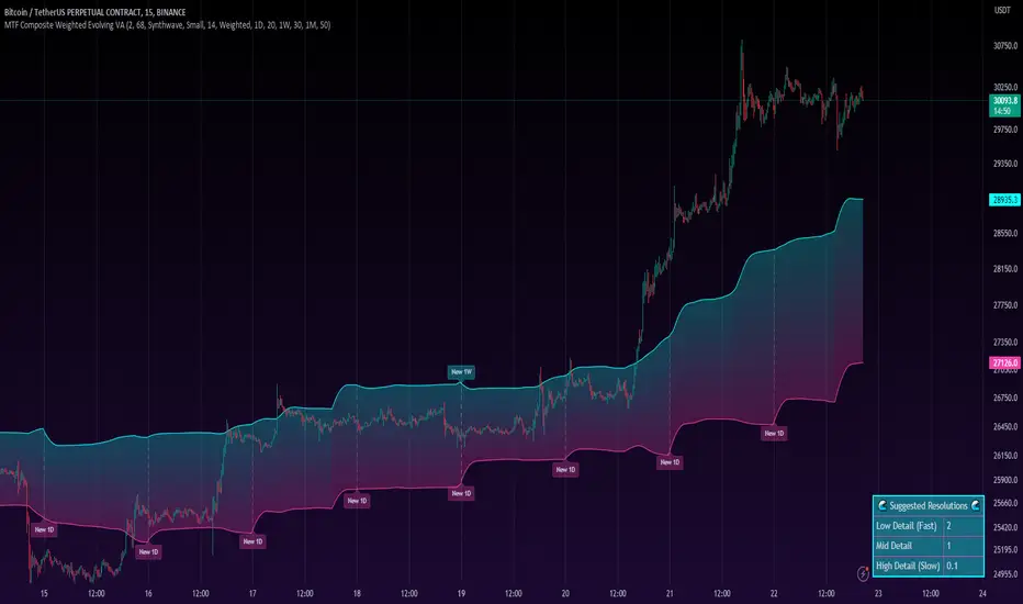
MTF Evolving Weighted Composite Value Area🧾 Description:
This indicator calculates evolving value areas across 3 different timeframes/periods and combines them into one composite, multi-timeframe evolving value area - with each of the underlying timeframes' VAs assigned their own weighting/importance in the final calculation. Layered with extra smoothing options, this creates an informative and useful 'rolling value area' effect that can give you a better perspective on the value area across multiple periods at once as it develops - without total calculation resets at the onset of every new period.
Let's start with a simplified primer on value areas and then jump in to the new ideas this indicator introduces.
🤔 What is a value area?
Value areas are a tool used in market profile analysis to determine the range of prices that represents where most trading activity occurred during a specific time period, typically within a single 'bar' of a certain higher timeframe, such as the 4-hour, daily, or weekly. It helps traders understand the levels where the market finds value.
To calculate the value area, we look at the distribution of prices and trading volume. We determine a percentage, usually 70% or 80%, that represents the significant portion of trading volume. Then, we identify the price range that contains this percentage of trading volume, which becomes the value area.
Value areas are useful because they provide insights into market dynamics and potential support and resistance levels. They show where traders have been most active and where they find value, and traders can use this information to make better-informed decisions.
For example, if price is trading within the value area, it suggests that it's within a range where traders see value and are actively participating, which could indicate a balanced market. If the price moves above or below the value area, it may signal a potential shift in market sentiment or a breakout/breakdown from the established range.
By understanding the value area, traders can identify potential areas of supply and demand, determine levels of interest for buyers and sellers, and make decisions based on the market's perception of value.
📑 Limitations of traditional value areas
Static representation: Value areas are usually represented as static zones calculated after the fact. For example, after a daily period is completed, a typical 1D VA indicator will display the value area for the past period with static horizontal lines. This approach doesn't give you the power to see how the value area evolved, or developed, during the time period, as it is only displayed retroactively. It also doesn't give you the ability to view it as it evolves in real-time. This is why we chose to use an evolving value area representation, specifically borrowed from @sourcey's Value Area POC/VAH/VAL script function for calculating evolving VAs.
Rollover resets - no memory of past periods!: The traditional value area is calculated over a static period - it is calculated from the beginning of the period, for example a 1 day period, to the end, and that's the end of it. When the next daily period begins, the calculation resets, and has no memory of the preceding period. This limits the usefulness of the value area visual when viewed near the beginning of a new period before price and volume have been given ample time to define an area.
Hard to absorb all of that information: Value areas aren't generally meant to be a hardline representation of something extremely exact - they're based on a percentage of the area where traders appeared to find value over a certain time period. Most traders use them as a guide for support and resistance levels or finding an expected range. Traders typically overlay multiple VAs - sometimes requiring several instances of the same indicator to be applied - to represent the VA across multiple timeframes such as the 4H, 1D, or 1W. The chart quickly gets cluttered and it's not necessarily easy to understand the relationship between these multiple periods' VAs at a glance.
🧪 New concepts introduced in this indicator
With the evolving weighted composite value area we tried to address these limitations, and we think the result can be useful and intuitive for traders who want more dynamic and practical VAs for their everyday technical analysis.
⚖️ 1. A composite, weighted multi-timeframe VA
This indicator's value areas represent a combination or composite of the value areas calculated across multiple timeframes. The VAs calculated across each timeframe are then given a weighting percentage, which determines their contribution to the final 'weighted composite value area'.
Pictured below: a 4H/1D/1W MTF evolving weighted composite VA on the BTCUSDT Perpetual Futures (Binance) 5 minute chart:
Traditionally, when traders wanted to get a view of where the majority of trading activity occurred over the past four hours, day, and week, they would need to apply three value area indicators (or sometimes one if it allows multiple custom timeframes), each set to a different period (4H, 1D, 1W). The chart gets cluttered quickly and the information is hard to absorb in one shot. Addressing this problem was the main impetus for creating this weighted composite process.
〰️ 2. Rolling and smoothed evolving VAs
Because the composite VA is calculated based on multiple period VAs, there is no one single point where the area calculation resets (unless all 3 selected timeframes happen to rollover on the same bar). This creates a 'rolling' effect that gives a sense of the progression of the VA as price transitions through the different underlying time periods, without the traditional 'jump' in calculations between periods.
Pictured below: a 1D/1W/1M MTF evolving weighted composite VA on the NQ futures 1H chart:
To help give even more of a sense of perspective and 'progression' of the VA, there are also smoothing options to even out the 'jumps' at period-rollover points.
✔️ What's it good for?
Smoothed, rolling, and evolving multi-timeframe VAs that give you a better real-time perspective of where traders are finding value across multiple time periods at once.
📎 References
1. @sourcey's Value Area POC/VAH/VAL script by adapting its f_poc(tf) function.
💠 Features:
A MTF evolving weighted composite value area based on 3 underlying VAs calculated across customizable timeframes
Aesthetic and flexible coloring and color theme styling options
Period-roller labels and options for ease-of-use and legibility
⚙️ Settings:
Calculation Decimal Resolution: This setting essentially determines how 'granular' the value area calculating process is. This value should be set to some multiple of the tick size/smallest decimal of the symbol's price chart. Eg. On BTCUSDT, the tick size/decimal is usually 0.1. So, you might use 0.5. On TSLA, the tick size is 0.01. You might use 0.05 or 0.25. Beware: if the resolution is too small, calculation will take too long and the script may timeout.
Show Me Suggested Resolutions: If enabled, a label will display in the bottom right of the chart with some suggested resolutions for the current chart.
Area Percentage: Set the displayed percentage of the calculated composite value area. Igor method = 70%; Daniel method: 68%.
Use a Color Theme: When this setting is enabled, all manual 'Bullish and Bearish Colors' are overridden. All plots will use the colors from your selected Color Theme - excepting those plots set to use the 'Single Color' coloring method.
Color Theme: When 'Use a Color Theme' is enabled, this setting allows you to select the color theme you wish to use.
Resistance Color: When 'Use a Color Theme' is disabled, this will set the 'resistance color' for the composite VA.
Support Color: When 'Use a Color Theme' is disabled, this will set the 'support color' for the composite VA.
Show Period Rollover Labels: When enabled, a label will show above or below the composite VA marking any underlying period rollovers with the label 'New __' (eg. 'New 4H', 'New 1D', 'New 1W').
Size: Sets the font size of the period rollover labels.
Show Period Rollover Lines: When enabled, a translucent vertical dashed line will be drawn across the composite VA when one of the underlying periods rolls over.
Fill Composite Value Area: When enabled, the composite VA will be filled with a gradient coloring from the support line to the resistance line using their respective colors.
Smooth: When enabled, a smoothing moving average will be applied to the composite value area.
Smoothing Period: Set the lookback period for the smoothing average.
Smoothing Type: Set the calculation type for the smoothing average. Options include: Exponential, Simple, Weighted, Volume-Weighted, and Hull.
Enable: Include/exclude a timeframe's VA in the composite VA calculation.
Timeframe: Set the timeframe for this specific underlying VA.
Weighting %: Set the weighting percentage or 'importance' of this timeframe's value area in calculating the composite VA. Beware! The sum of the weighting percentages across all enabled timeframes must ALWAYS add up to 100 in order for this indicator to work as designed.
[Pt] Periodic Volume ProfileThis script is an attempt to recreate the Periodic Volume Profile that is built-in by TradingView, with slightly different features. Related blog: www.tradingview.com
This script is based on another script "Volume Profile, Pivot Anchored" by @dgtrd
*Note that only limited number Volume Profile can be displayed on the chart due to limitations on displaying boxes and lines.
Description
This Periodic Volume Profile (PVP) indicator allows trades to view volume profiles for periods longer than the current timeframe. The indicator builds one general volume profile for each new period, set by the user through the “Periodic Timeframe” input parameter.
This script also has the option to extend Point of Control (POC) lines with optional end conditions: Until Bar Touch, Until Last Bar, Until Bar Cross, or None, which extends to the right.
Signals are generated for Naked POC touches and crosses by a triangle symbol and a cross symbol, by default.
Alerts are available for POC touches and crosses.
What is Volume Profile?
Volume profile is a technical analysis tool that shows the volume of trades at different prices for a given security or market over a specific period of time.
Volume profile can be used to identify key levels of support and resistance, as well as to assess the overall supply and demand for a security. For example, if there is a high volume of trades at a particular price level, this may indicate that there is a significant level of support or resistance at that price. On the other hand, if there is relatively low volume at a particular price, this may indicate that there is not much interest in trading at that level.
Traders can use volume profile to identify trends, make trading decisions, and set stop-loss and take-profit orders. It can also be useful for identifying patterns such as "pockets of liquidity," which are areas where there is a high volume of trades but relatively little price movement.
It is important to note that volume profile should be used in conjunction with other technical analysis tools and should not be relied upon in isolation. It is also important to consider the overall context and market conditions when interpreting volume profile data.
Key Difference with TradingView's PVP indicator - TradingView's PVP intraday period does not align with standard intraday timeframes as it is determined by # of bars. This script provides volume profiles that aligns with higher timeframe periods.
Enjoy~!
Visible Range Mean Deviation Histogram [LuxAlgo]This script displays a histogram from the mean and standard deviation of the visible price values on the chart. Bin counting is done relative to high/low prices instead of counting the price values within each bin, returning a smoother histogram as a result.
Settings
Bins Per Side: Number of bins computed above and below the price mean
Deviation Multiplier: Standard deviation multiplier
Style
Relative: Determines whether the bins length is relative to the maximum bin count, with a length controlled with the width settings to the left.
Bin Colors: Bin/POC Lines colors
Show POCs: Shows point of controls
Usage
Histograms are generally used to estimate the underlying distribution of a series of observations, their construction is generally done taking into account the overall price range.
The proposed histogram construct N intervals above*below the mean of the visible price, with each interval having a size of: σ × Mult / N , where σ is the standard deviation and N the number of Bins per side and is determined by the user. The standard deviation multipliers are highlighted at the left side of each bin.
A high bin count reflects a higher series of observations laying within that specific interval, this can be useful to highlight ranging price areas.
POCs highlight the most significant bins and can be used as potential support/resistances.
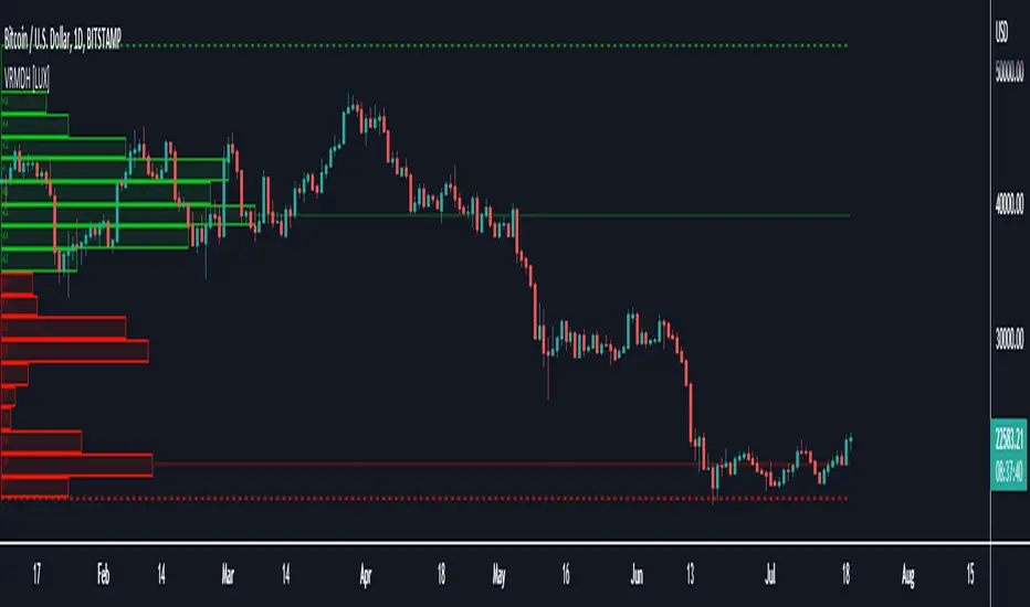
Volume ProfileThis is a Volume Profile based on pine script arrays.
The main idea behind this script is from the user @IldarAkhmetgaleev .
He created an awesome piece of code for free users on tradingview.
Here are some changes to the main script:
0. Used Pine Script Arrays for doing/storing calculations.
1. The bar labels are replaced with lines.
2. Added a POC line.
3. Bar growing directions changed from right to left.
4. Added an option to change bar width.
Inputs:
0. Volume Lookback Depth : Number of bars to look back for volume calculations.
1. Bar Length Multiplier : Bar length multiplier to make bar long or short.
2. Bar Horizontal Offset : Horizontal distance from the current bar in the right direction.
3. Bar Width : Width of the bars.
4. Show POC Line : Show or hide the POC line.
Happy trading.
AMT VWAP [hardi]█ OVERVIEW
AMT VWAP is a clean, minimalist VWAP indicator with Standard Deviation bands, designed to complement the Auction Market Theory (AMT) trading methodology by Fabio Valentino.
This indicator focuses on one thing and does it well: displaying VWAP and its deviation bands clearly on your chart.
█ FEATURES
- Daily VWAP with automatic reset
- ±1 Standard Deviation bands (cyan)
- ±2 Standard Deviation bands (orange) - extreme zones
- Clean labels that don't clutter your chart
- Info table showing current bias and zone
- Compact Mode for mobile/smartphone users
- Fully customizable colors and settings
- Built-in alerts for all levels
█ HOW TO USE
VWAP (Volume Weighted Average Price) represents the "fair value" where most volume has transacted. In AMT methodology:
BIAS DETERMINATION:
- Price ABOVE VWAP = Bullish bias (buyers in control)
- Price BELOW VWAP = Bearish bias (sellers in control)
TRADING ZONES:
- ±1 SD: Normal deviation zone - potential mean reversion area
- ±2 SD: Extreme zone - high probability reversal area (95%+ reversion rate)
ENTRY STRATEGIES:
1. Trend Following: Buy pullbacks to VWAP in uptrend, sell rallies to VWAP in downtrend
2. Mean Reversion: Fade moves at ±2 SD bands with confirmation
█ RECOMMENDED SETUP
Use this indicator together with:
- TradingView's built-in "SVP HD" (Session Volume Profile) for POC/VAH/VAL levels
- AMT CVD indicator (companion indicator) for order flow analysis
This combination gives you the complete AMT toolkit:
- SVP HD → Key levels (POC, VAH, VAL)
- AMT VWAP → Dynamic support/resistance & bias
- AMT CVD → Aggression, Absorption, Exhaustion signals
█ SETTINGS
Display Settings:
- Compact Mode - Enable for cleaner mobile view
- Show Labels - Toggle level labels
- Label Size - Adjust for your screen
VWAP Settings:
- Band Multipliers - Adjust SD band distance (default: 1.0 and 2.0)
- Colors - Fully customizable
- Line widths - Adjust visibility
Alerts:
- Near VWAP
- Near ±1 SD
- Near ±2 SD (extreme zones)
█ METHODOLOGY
This indicator is based on Auction Market Theory as taught by Fabio Valentino:
"The market is a continuous auction seeking fair value. VWAP represents this fair value dynamically throughout the session. Deviations from VWAP create trading opportunities as price tends to revert to the mean."
Key principles:
- Read, don't predict
- Location over technique
- Evidence-based entries
█ ALERTS
Set alerts for:
- Price approaching VWAP (potential support/resistance)
- Price at ±1 SD (first deviation - watch for reaction)
- Price at ±2 SD (extreme - high probability reversal zone)
█ NOTES
- Works on all timeframes
- Best used on 15m for intraday entries
- VWAP resets daily at market open
- Combine with volume profile for best results
█ CREDITS
Based on Auction Market Theory methodology by Fabio Valentino.
Indicator developed for the trading community.
If you find this useful, please leave a like! 👍
vwap, volume-weighted-average-price, standard-deviation, bands, auction-market-theory, amt, fabio-valentino, mean-reversion, trend-following, intraday, day-trading, support-resistance, fair-value

AMT CVD [hardiman]█ OVERVIEW
AMT CVD is a Cumulative Volume Delta indicator with a unique numeric labeling system designed for the Auction Market Theory (AMT) methodology by Fabio Valentino.
Instead of just showing CVD as a line, this indicator displays numeric labels (+3, +2, +1, 0, -1, -2, -3) and "A" for Absorption, making it easy to identify the current phase of the AMT workflow at a glance.
█ KEY FEATURES
• CVD with numeric aggression labels (+3 to -3)
• "A" label for Absorption detection (high volume + price stagnation)
• Automatic Exhaustion detection (aggression fading)
• Entry signal markers (L for Long, S for Short)
• Real-time workflow dashboard
• Compact Mode for mobile users
• Customizable thresholds and colors
• Built-in alerts for each phase
█ THE NUMERIC LABEL SYSTEM
BUYER AGGRESSION:
• +3 = Extremely aggressive buying (delta > 3.5x average)
• +2 = Strong buying pressure (delta > 2.5x average)
• +1 = Mild buying pressure (delta > 1.5x average)
SELLER AGGRESSION:
• -1 = Mild selling pressure (delta > 1.5x average)
• -2 = Strong selling pressure (delta > 2.5x average)
• -3 = Extremely aggressive selling (delta > 3.5x average)
SPECIAL LABELS:
• 0 = Neutral / Exhaustion (no significant aggression)
• A = Absorption (high volume but price doesn't move)
█ AMT WORKFLOW
The indicator tracks the complete AMT entry workflow:
1️⃣ AGGRESSION → Look for +2/+3 or -2/-3 labels
2️⃣ ABSORPTION → Wait for "A" label (price held despite aggression)
3️⃣ EXHAUSTION → Watch labels decrease toward 0
4️⃣ ENTRY → Reversal label appears (direction change)
SHORT SETUP EXAMPLE (at resistance):
+1 → +2 → +3 → A → A → +1 → 0 → -1 → ENTRY SHORT
LONG SETUP EXAMPLE (at support):
-1 → -2 → -3 → A → A → -1 → 0 → +1 → ENTRY LONG
█ DASHBOARD
The dashboard shows real-time status:
• Stage: Current workflow phase (1-5)
• Aggression: Current numeric level
• Absorption: ✓ NOW / ○ RECENT / ✗ NONE
• Exhaustion: ✓ YES / ○ NO
• Signal: WAIT / WATCH / READY / LONG / SHORT
█ HOW TO USE
1. Add this indicator to a separate pane below your chart
2. Use TradingView's built-in SVP HD for key levels (POC/VAH/VAL)
3. Add AMT VWAP for bias determination
4. Wait for price to reach a key level
5. Watch the CVD labels for the AMT sequence
6. Enter when the dashboard shows "READY" or entry signal appears
█ RECOMMENDED SETUP
Complete AMT toolkit:
• Main Chart: SVP HD (built-in) + AMT VWAP
• Lower Pane: AMT CVD (this indicator)
Timeframes:
• Higher TF (H1/H4): Identify structure and key levels
• Entry TF (15m): Execute using this CVD indicator
█ SETTINGS
Display:
• Compact Mode - Simplified view for mobile
• Show Numeric Labels - Toggle the +3/-3 labels
• Label Size - Adjust for your preference
• Dashboard Position - Move to any corner
CVD Settings:
• Relative Length - Period for threshold calculation (default: 20)
• Threshold 1/2/3 - Multipliers for aggression levels
Absorption:
• Volume Multiplier - How much above average = high volume (default: 1.5x)
• Price Threshold - Max price change % for absorption (default: 0.1%)
Colors:
• Fully customizable for buyer/seller/absorption
█ ALERTS
• Absorption Detected - "A" label appears
• Exhaustion Detected - Aggression fading to 0
• Long Entry Signal - Full sequence complete for long
• Short Entry Signal - Full sequence complete for short
█ IMPORTANT NOTES
⚠️ CVD APPROXIMATION: This indicator approximates volume delta from OHLC data. For more accurate CVD, consider using exchange-native order flow tools or Volume Suite by Leviathan as a reference.
⚠️ CONFIRMATION REQUIRED: Signals should be confirmed with:
• Price at key level (VAH/VAL/POC)
• Visual rejection (wicks)
• Higher timeframe bias alignment
█ METHODOLOGY
Based on Auction Market Theory by Fabio Valentino:
"Don't predict, READ the market. Wait for evidence: Aggression → Absorption → Exhaustion → then Execute."
Core principles:
• Location is more important than technique
• Be wrong immediately (tight stops at invalidation)
• Evidence-based entries only
█ CREDITS
Based on Auction Market Theory methodology by Fabio Valentino.
Designed for traders who want a systematic, evidence-based approach.
If this helps your trading, please leave a like! 👍
Questions? Drop a comment below.
```
---
## TAGS (for TradingView)
```
cvd, cumulative-volume-delta, volume-delta, order-flow, auction-market-theory, amt, fabio-valentino, absorption, exhaustion, aggression, entry-signal, day-trading, intraday, volume-analysis, delta
```
---
## CATEGORY
```
Volume
```

Multi-Timeframe Volume Profile - Auto HVN WallsMulti-Timeframe Volume Profile - Auto HVN Walls
Overview This indicator provides a highly flexible Volume Profile solution that operates across multiple timeframes (Session, Weekly, Monthly, Yearly). Unlike standard profiles, this tool features a unique "Auto HVN Wall" detection system. It automatically identifies meaningful High Volume Nodes (HVNs) within the profile structure and extends them forward as potential support and resistance zones, creating a dynamic map of market structure as it develops.
Key Features
Multi-Timeframe Support: Switch seamlessly between Session, Weekly, Monthly, and Yearly profiles.
Auto HVN Walls (Structure Detection): The script analyzes the profile shape in real-time. When it detects significant clusters of volume (HVNs), it automatically draws extended lines ("walls"). These walls often act as magnets or support/resistance levels where price has previously found acceptance.
Session Filtering: When in "Session" mode, you can define specific time windows (e.g., 0930-1615) to isolate Regular Trading Hours (RTH) volume, ignoring overnight data.
Auto-Scaling Width (Monthly Mode): For Monthly profiles, the histogram width dynamically changes throughout the month. It starts wide at the beginning of the month to be visible and gradually narrows as the month progresses, keeping your chart clean.
High Precision: Uses lower timeframe data (user-selectable) to build the profile, ensuring accuracy even on higher timeframe charts.
Alerts: Built-in alert conditions for price crossing the developing POC, VAH, or VAL.
How It Works
Data Accumulation: The script fetches lower timeframe volume and price data (e.g., 5-minute data on a 1-hour chart) to construct a precise volume histogram.
Wall Detection: It runs a smoothing algorithm over the volume profile. If a price level accumulates volume significantly higher than the average (controlled by the Volume Threshold Multiplier), it marks that level as a "Wall" and extends it.
Value Area: Standard Value Area High (VAH), Value Area Low (VAL), and Point of Control (POC) are calculated and displayed for the selected period.
Settings Guide
Profile Period: Choose between Session, Weekly, Monthly, or Yearly.
Session Time: (Only active in "Session" mode) Define the start and end times for the profile (e.g., 0930-1615).
Calculation Precision: Determines the lower timeframe used to build the profile. Lower is more precise but may load slower.
The Walls:
Smoothing Factor: How much to smooth the volume data before finding walls. Higher = fewer, more significant walls.
Volume Threshold: How much volume is needed to trigger a wall.
Extend Walls: If checked, walls extend infinitely to the right.
Auto-Scale Width: (Monthly Only) dynamically adjusts the profile width based on the day of the month.
Use Case This tool is ideal for auction market theorists and volume profile traders who want to visualize where value is building in real-time and identify "sticky" price levels (Walls) where the market is likely to rotate or consolidate.
Disclaimer This script and the information presented here are for educational and informational purposes only. They do not constitute financial advice, investment recommendations, or trading signals. Trading in financial markets involves a significant risk of loss and is not suitable for all investors. Past performance of any trading system or methodology is not necessarily indicative of future results. Use this tool at your own discretion and risk.

Custom Weekly Volume Profile [Multi-Timeframe]Description: This indicator renders a high-precision Weekly Volume Profile that resets at the start of every trading week. Unlike standard fixed-range profiles, this script builds the profile bar-by-bar using lower timeframe data (e.g., 1-minute or 5-minute data) to ensure accuracy even on higher timeframe charts.
It is designed for traders who track the developing value of the current week (Auction Market Theory) and need specific alerts when price tests the edges of value.
Key Features:
Developing Weekly Profile:
The profile resets automatically at the beginning of the week (Sunday/Monday).
It tracks the Point of Control (POC), Value Area High (VAH), and Value Area Low (VAL) in real-time as the week progresses.
Previous Week Levels:
The script automatically stores the final levels (POC, VAH, VAL) of the previous week and projects them forward. This allows you to trade tests of the prior week's value.
Auto-Scaling Histogram:
Smart Width: The profile starts wider at the beginning of the week (when data is sparse) and automatically shrinks as the week progresses (Thursday/Friday) to keep your chart clean and readable.
Advanced Alerting:
Crossover Alerts: Trigger alerts when price crosses the developing VAH/VAL or the previous week's levels.
Time Window Filter: Includes a session input (default 08:30-15:00) to restrict alerts to specific trading hours, preventing notifications during low-volume overnight sessions.
Customization:
Precision: Adjustable "Row Size" and "Calculation Timeframe" to tune performance vs. accuracy.
Visuals: Full color control over the Value Area, Outer Volume, and Level Lines.
Settings:
Calculation Precision: Determines the lower timeframe used to calculate the volume (e.g., set to "5" for 5-minute precision).
Value Area %: Default is 70%, standard for AMT trading.
Timezone: Adjustable to ensure the weekly reset aligns with your local exchange time (e.g., America/Chicago for CME Futures).
Disclaimer: This script is for educational and informational purposes only. It does not constitute financial advice, trading recommendations, or a solicitation to buy or sell any financial instrument. Trading futures and other financial markets involves significant risk and is not suitable for every investor. Past performance of any trading system or methodology is not necessarily indicative of future results. The user assumes all responsibility for any trading decisions made based on the information provided by this tool. Use at your own risk.

Harmonic Liquidity Waves [JOAT]Harmonic Liquidity Waves
Overview
Harmonic Liquidity Waves is an open-source oscillator indicator that combines multiple volume-based analysis techniques into a unified liquidity flow framework. It integrates VWAP calculations, Chaikin Money Flow (CMF), Money Flow Index (MFI), and Klinger Volume Oscillator (KVO) with custom harmonic wave calculations to provide a comprehensive view of volume dynamics and money flow.
What This Indicator Does
The indicator calculates and displays:
Liquidity Flow - Volume-weighted price movement accumulated over a lookback period
Harmonic Wave - Multi-depth smoothed oscillator derived from liquidity flow
Chaikin Money Flow (CMF) - Classic accumulation/distribution indicator
Money Flow Index (MFI) - Volume-weighted RSI showing buying/selling pressure
Klinger Volume Oscillator (KVO) - Trend-volume relationship indicator
Wave Interference - Combined constructive/destructive wave patterns
Volume Profile POC - Point of Control from simplified volume distribution
How It Works
The core liquidity flow calculation tracks volume-weighted price changes:
calculateLiquidityFlow(series float vol, series float price, simple int period) =>
float priceChange = ta.change(price)
float volumeFlow = vol * math.sign(priceChange)
// Accumulated over period using buffer array
float avgFlow = flowSum / period
avgFlow
The harmonic oscillator applies multi-depth smoothing:
harmonicOscillator(series float flow, simple int depth, simple int period) =>
float harmonic = 0.0
for i = 1 to depth
float wave = ta.ema(flow, period * i) / i
harmonic += wave
harmonic / depth
CMF measures accumulation/distribution using the Money Flow Multiplier:
float mfm = ((close - low) - (high - close)) / (high - low)
float mfv = mfm * vol
float cmf = ta.sum(mfv, period) / ta.sum(vol, period) * 100
Signal Generation
Liquidity shift signals occur when:
Bullish Shift: Smoothed wave crosses above signal line
Bearish Shift: Smoothed wave crosses below signal line
Strong signals require volume indicator confirmation:
Strong Bull: Bullish shift + CMF > 0 + MFI > 50 + KVO > 0
Strong Bear: Bearish shift + CMF < 0 + MFI < 50 + KVO < 0
Divergence detection compares price pivots with liquidity wave pivots to identify potential reversals.
Dashboard Panel (Bottom-Right)
Wave Strength - Normalized wave magnitude
Volume Pressure - Current volume vs average percentage
Flow Direction - BUYING or SELLING based on wave sign
Histogram - Wave minus signal line value
CMF - Chaikin Money Flow reading
MFI - Money Flow Index value (0-100)
KVO - Klinger oscillator value
Vol Confluence - Combined volume indicator score
Signal - Current actionable status
Visual Elements
Liquidity Wave - Main oscillator line
Wave Signal - Smoothed signal line for crossover detection
Wave Histogram - Difference between wave and signal
Wave Interference - Area plot showing combined wave patterns
CMF/KVO/MFI Lines - Individual volume indicator plots
Divergence Labels - BULL DIV / BEAR DIV markers
Shift Markers - Triangles for basic shifts, labels for strong shifts
Input Parameters
Wave Period (default: 21) - Base period for liquidity calculations
Volume Weight (default: 1.5) - Multiplier for volume emphasis
Harmonic Depth (default: 3) - Number of smoothing layers
Smoothing (default: 3) - Final wave smoothing period
Suggested Use Cases
Identify accumulation/distribution phases using CMF and wave direction
Confirm momentum with MFI overbought/oversold readings
Watch for divergences between price and liquidity flow
Use strong signals when multiple volume indicators align
Timeframe Recommendations
Best on 15m to Daily charts. Volume-based indicators require sufficient trading activity for meaningful readings.
Limitations
Volume data quality varies by exchange and instrument
Divergence detection uses pivot-based lookback and may lag
Volume Profile POC is simplified and not a full profile analysis
Open-Source and Disclaimer
This script is published as open-source under the Mozilla Public License 2.0 for educational purposes. It does not constitute financial advice. Past performance does not guarantee future results. Always use proper risk management.
- Made with passion by officialjackofalltrades
