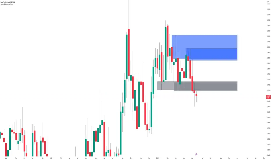
Support & Resistance ZonesTitle: A Comprehensive Guide to the Support & Resistance Zones Indicator
Introduction
In the world of technical analysis, the Support & Resistance Zones indicator plays a crucial role in identifying potential trading opportunities. These zones are essential for traders looking to capitalize on bounces or break and retests. In this article, we will delve into the specifics of the Support & Resistance Zones indicator, outlining how it works, how it finds and marks zones, and the various options available for traders.
What the indicator is about
The Support & Resistance Zones indicator, developed by @HarryCTC, is a powerful tool for detecting areas of potential price reversal or consolidation in a financial market. These zones are significant as they can act as a guide for traders to make informed decisions on entering or exiting positions. Specifically, the indicator helps identify:
1. Support Zones: Areas where the price has a tendency to bounce back up after falling, indicating a potential buying opportunity.
2. Resistance Zones: Areas where the price has a tendency to reverse after rising, indicating a potential selling opportunity.
How the indicator finds its zones
The Support & Resistance Zones indicator utilizes pivot points to identify potential support and resistance levels. By analyzing the fractal structure of the price chart, the indicator identifies key turning points, known as bull and bear fractals. The bull fractal is a high pivot point, while the bear fractal is a low pivot point.
The fractal structure is determined by the 'Switch Zone Period' input, which can be adjusted to suit the trader's preferences. A higher value will result in fewer zones being identified, while a lower value will result in more zones.
How it marks zones and why it marks zones
The indicator marks the support and resistance zones by creating rectangular boxes around the identified fractal points. The zones are extended horizontally from the fractal point, allowing traders to visualize the potential areas of price reversal.
The zones are marked for the following reasons:
1. To provide a clear visual representation of potential support and resistance levels.
2. To help traders identify potential entry and exit points based on the price's reaction to these zones.
3. To serve as a reference for stop-loss and take-profit levels when planning trades.
The indicator's for traders trading bounces or break and retests
Traders who focus on trading bounces or break and retests can benefit immensely from the Support & Resistance Zones indicator. By providing a visual representation of key support and resistance levels, the indicator enables traders to:
1. Identify potential buying opportunities at support zones where the price is likely to bounce back up.
2. Identify potential selling opportunities at resistance zones where the price is likely to reverse after rising.
3. Make informed decisions on stop-loss and take-profit levels based on the price's proximity to support and resistance zones.
4. Monitor the market for potential breakouts or breakdowns when the price breaches these zones.
Indicator options
The Support & Resistance Zones indicator offers several customizable options to suit the trader's preferences. These options include:
1. Switch Zone Period: Adjusts the number of periods used to calculate the fractal structure, influencing the number of identified zones.
2. No. of Displayed Zones: Determines the maximum number of zones displayed on the chart, ranging from 1 to 8.
3. Zone Extension: Adjusts the horizontal extension of the support and resistance zones.
4. Resistance Zone Color: Customizes the color of the resistance zone boxes.
5. Support Zone Color: Customizes the color of the support zone boxes.
6. Zone Border Color: Customizes the color of the zone box borders.
Conclusion
The Support & Resistance Zones indicator is a valuable tool for traders looking to identify potential trading opportunities based on the price's interaction with support and resistance levels. By providing a clear visual representation of these zones, the
indicator allows traders to make informed decisions on entry and exit points, stop-loss, and take-profit levels. With customizable options, the indicator can be tailored to suit individual trading preferences and strategies.
ابحث في النصوص البرمجية عن "zone"
Supply Demand Zones ProSupply Demand Zones PRO
Version: 1.0
Built with: Pine Script v6
________________________________________
🧭 HOW TO USE Start Here
🧠 What it does default behavior
• ✅ Automatically identifies Supply & Demand zones on your chart
• ✅ Automatically ranks each zone from 0 to 10 higher = stronger
• ✅ Works across most TradingView symbols and timeframes with default settings
⚙️ Default settings recommended for most instruments
Use the default settings for:
• 💱 Forex
• 🪙 Crypto
• 📊 Indices
• 🛢️ Commodities
• 🏛️ Stocks
Defaults are tuned to provide a balanced mix of quality zones + clean charts.
🎯 How to trade with it high-level workflow
1. 🥇 Prioritize strong zones
o Focus on higher scores commonly 7–10 for best reversal potential.
2. 🔄 Wait for a reversal setup at the zone
o Example triggers: rejection wick, engulfing candle, strong reaction candle, structure shift.
3. ✅ Confirm with other indicators before entering
o Use confirmation tools (your choice), such as:
📈 Trend filter (MA / market structure)
🧪 Momentum (RSI / Stoch / MACD)
📉 Volume / volatility tools
o Then take BUY from demand or SELL from supply *only when confirmation aligns
🧩🖤 Executive Summary: PRO Features Overview
The Supply Demand Zones PRO indicator is a professional-grade tool built on the latest Pine Script v6, designed to automatically identify and score high-probability supply and demand zones.
It moves beyond simple zone plotting by incorporating a suite of advanced features that provide a deeper, more actionable market context. This helps traders filter out noise, focus on significant levels, and make more informed decisions.
The indicator is universally compatible and works seamlessly across all major asset classes and timeframes:
• Forex: EURUSD, GBPUSD, USDJPY
• Commodities: Gold/XAUUSD, Silver, Oil
• Indices: NQ, ES, DAX, FTSE
• Cryptocurrencies: Bitcoin, Ethereum, Altcoins
• Stocks: Individual equities
Most symbols available on TradingView are fully supported.
Notice on repainting 🕯️⬛
Active zones won’t repaint unless they are invalidated. Gray/Historic zones may repaint, and that’s fine—this script only displays the most recent and stronger historic zones (if historic zones are enabled).
________________________________________
⬛🛠️Key PRO Features Overview
⚙️ Feature 📌 Description
Zone Strength Ranking ||| Each zone is dynamically scored from 1–10 based on its age and number of retests. Fresher, less-tested zones are stronger, helping prioritize high-impact levels.
Real-Time Distance ||| Each active zone’s info label shows the exact distance (in pips) from current price to the zone edge for quick risk/opportunity assessment.
Trading Session Tracking ||| Zones are tagged by formation session (Asian / London / New York) for added context—high-volume session zones often matter more.
Automated Retest Markers ||| The script tracks retests and places an “R” marker for each retest, giving a clear visual history of price interaction.
Advanced ATR Filtering ||| Volatility-based filters control zone quality: set min/max zone height and optionally enforce a consistent zone height using ATR.
Minimum Zone Distance ||| Reduces clutter by requiring a minimum number of bars between new zones, ensuring zones are distinct and well-separated.
Dual Label Controls Independently toggle info labels for Active vs Historic zones to keep charts clean while preserving key detail.
Built on Pine Script v6 ||| Uses the newest Pine Script version for better efficiency, reliability, and smoother handling of complex logic/drawings.
________________________________________
Detailed Feature Breakdown ⬛
Zone Strength Ranking ⬛
The strength score is a proprietary calculation that helps traders instantly gauge the potential of a supply or demand zone. It is calculated in real time using:
1. Age of the Zone: As zones age, they may lose relevance. Strength decreases as the number of bars since creation increases.
2. Number of Retests: The first test is often the highest-probability reaction. Each retest reduces strength as liquidity is absorbed.
✅ A high score (7/10+) indicates a fresh, less-tested zone that may produce a strong reaction.
⚠️ A low score suggests a zone is old and/or heavily tested—use extra caution.
________________________________________
🧱⬛Invalidation & Historic Zones
A zone becomes invalidated broken when price closes beyond its outer boundary or wicks beyond it, depending on settings. Once broken, it becomes a Historic Zone and turns gray.
This matters for structure: a broken supply zone can become future demand a flip zone, and vice versa.
________________________________________
🧪⬛Advanced Filtering Explained
Three ATR-based filters control zone quality:
• Max Zone Height (ATR Multiplier): Blocks zones that are too large to trade effectively. Example: 1.0 ignores zones taller than 1× ATR.
• Min Zone Height (ATR Multiplier): Filters out zones that are too thin and likely noise. Example: 1.0 rejects zones smaller than 1× ATR.
• Force Zone Height (ATR Multiplier): Normalizes zone heights by expanding smaller valid zones up to the minimum ATR target. Example: 1.0 expands zones to at least 1× ATR.
________________________________________
🧾⬛Configuration Guide
⚙️⬛Zone Detection
⚙️ Setting 🔧 Default 📝 Description
Swing Length (Sensitivity) 12 Lookback bars for pivot high/low detection. Higher = fewer, stronger zones.
Max Zones to Display 10 Max number of active Supply + Demand zones shown.
Max Zone Height (ATR) 1.0 Rejects zones taller than this ATR multiplier.
Min Zone Height (ATR) 1.0 Rejects zones smaller than this ATR multiplier.
Force Zone Height (ATR) 1.0 Expands valid zones to be at least this ATR multiplier.
Min Distance Between Zones 44 Minimum bars required between consecutive zones of the same type.
________________________________________
🧱⬛Zone Settings
⚙️ Setting 🔧 Default 📝 Description
Zone Invalidation Close “Close” = candle must close past zone; “Wick” = wick past zone breaks it.
Show Historic Zones On Toggles visibility of broken (historic) zones.
Active Zones Lookback 1000 Hides active zones older than this many bars.
Historic Zones Lookback 1000 Hides historic zones older than this many bars.
________________________________________
🖥️⬛Display
⚙️ Setting 🔧 Default 📝 Description
Show Active Zone Info On Toggles text labels for active (unbroken) zones.
Show Historic Zone Info Off Toggles text labels for historic (broken) zones.
Label Size Small Adjusts the font size of zone info labels.

Interest ZonesThis indicator automatically identifies and plots "Interest Zones" around significant pivot highs and lows, representing potential areas of institutional interest, support/resistance, or accumulation/distribution. Zones are dynamically merged when pivots cluster near the same price level and extended for visibility.
How It Works (Technical Methodology)
Pivot Point Detection
The indicator uses Pine Script's ta.pivothigh() and ta.pivotlow() with asymmetric left/right lengths (default left=20, right=13) to detect swing highs and lows. This allows for customizable sensitivity – longer left for stronger confirmation, shorter right for faster detection.
Zone Start Condition (Filtering)
Multiple modes control from which point in history zones begin to be drawn:
"None": All historical pivots (limited by max zones).
"Auto (Start of Day)": Zones only from the beginning of the current trading day (resets daily).
"Manual Date": User-defined fixed date.
"Interactive (Chart)": User-confirmed date via input (useful for backtesting specific periods).
"Last X Bars": Only pivots within the last user-defined number of bars (default 400).
A vertical line marks the start point in date-based modes for visual reference.
Zone Construction
For each valid pivot:
Zone thickness is based on ATR(14) × user-defined multiplier (default 0.3) for dynamic, volatility-adjusted height.
Pivot High zones: Centered below the high (potential supply/resistance).
Pivot Low zones: Centered above the low (potential demand/support).
Zones are drawn as boxes extending to the right, with gray fill and border.
Merge & Overlap Logic
When a new pivot falls inside an existing zone or is very close (within user-defined "Proximity Sensitivity %" of the zone's midpoint, default 1.1%):
The new pivot is merged into the existing zone.
A counter ("x2", "x3", etc.) is displayed on the zone, indicating how many pivots have clustered there.
The zone is strengthened visually (counter text) and extended further right.
This highlights high-interest levels where price repeatedly reversed.
Zone Management
In "None" mode: Only the most recent user-defined max zones are kept (default 5) – oldest deleted automatically.
In other modes: Up to ~490 zones (performance limit), oldest pruned if exceeded.
All zones auto-extend to the right on the last bar for continuous visibility.
Visual Elements
Uniform gray color for all zones (configurable).
Transparent background fill (adjustable).
Counter text in white (configurable) when zones have multiple touches.
Clean, non-directional design – focuses purely on clustered reversal points.
How to Use
Interest Zones highlight price levels where the market has shown repeated respect through multiple swing pivots – often coinciding with institutional order clusters, psychological levels, or hidden support/resistance.
Higher counter values ("x3+", "x5+"): Stronger zones – higher probability of reaction on retest.
Use for:
Potential reversal or bounce areas when price approaches a zone.
Confluence with other tools (order blocks, FVG, volume profile, etc.).
Stop-loss placement beyond zones or take-profit at opposite zones.
Daily reset ("Auto Start of Day"): Ideal for intraday trading – fresh zones each session.
Backtesting: Use "Manual" or "Interactive" date modes to analyze specific historical periods.
"Last X Bars": Good for medium-term swing analysis without full history clutter.
Adjust ATR multiplier for tighter (lower) or wider (higher) zones based on asset volatility. Increase proximity sensitivity for more aggressive merging in ranging markets.
Combine with trend direction, volume, or higher-timeframe structure for best results.
Disclaimer
This indicator is a technical analysis tool and should be used in conjunction with other forms of analysis. Past performance does not guarantee future results. Always use proper risk management.

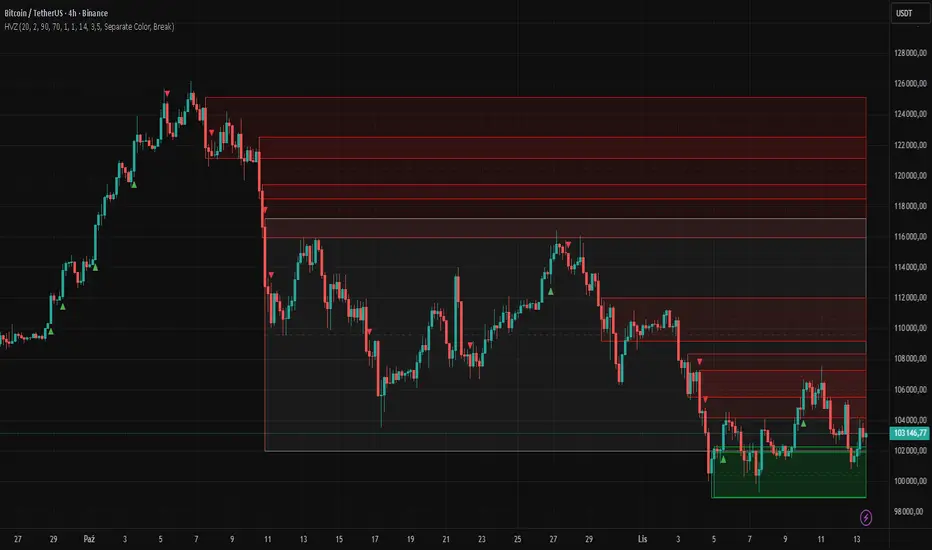
High Volume Zones with Signals – HVZ█ OVERVIEW
"High Volume Zones with Signals – HVZ" is a technical analysis indicator that identifies High Volume Zones (HVZ) on the chart and draws them as fully customizable boxes. Perfect for traders using price action, ICT, and Smart Money Concepts. The indicator highlights key volume-based support/resistance levels, detects potential consolidation zones (very large candles), and generates precise breakout and exit signals. Flexible volume filters, ATR filter, and visual styling options ensure a clean and highly effective chart.
█ CONCEPTS
The indicator detects candles with volume significantly above the average (default ≥ 2× SMA of volume over 20 periods). Such candles often signal institutional activity and create strong supply/demand zones.
The ATR filter additionally identifies very large candles – frequently a sign of market capitulation (panic buying/selling). Within the range of such a candle, prolonged consolidation often occurs, especially on higher timeframes (e.g., 4H and above).
Why are HVZ important? High-volume zones are areas where the market has left a large number of orders – institutions return there to “refresh” liquidity before the next move. A breakout against the zone’s character triggers a Break signal:
- Bullish HVZ broken downward (close below the lower boundary) → Break Down (sell),
- Bearish HVZ broken upward (close above the upper boundary) → Break Up (buy).
Note: The indicator requires real exchange volume – it will not work correctly on instruments without reported volume (e.g., certain CFDs or forex).
█ FEATURES
- HVZ Detection: Automatic identification of high-volume zones with Volume SMA Length and Volume Multiplier filters; historical initialization up to 500 candles back.
- ATR Filter: Optional detection of very large candles (potential consolidation/capitulation) using - ATR Length and ATR Multiplier; three action modes:
Skip Zone – large candle creates no zone,
Separate Color – zone is drawn in a distinct style (gray by default),
Normal Zone – treated like a regular HVZ.
- Gray zones (large candles, Separate Color): generate exactly the same Break signals as regular zones – based solely on the original candle direction (bullish → Break Down on lower break, bearish → Break Up on upper break). Gray color is only a visual marker for potential consolidation/capitulation zones.
- Customizable Boxes: Separate styles for bullish and bearish zones (border color, background gradient, line thickness and style); adjustable background and 50 % midline transparency.
- Break & Exit Signals:
Break Up/Down – green/red triangle after a candle closes outside the zone (zone disappears, triangle remains as a trace).
Exit Up/Down – green/red circle when price leaves the zone without a full breakout.
Signal Type option: Break, Exit, or Both.
- Midline: Automatic dashed line at the 50 % zone level with independent transparency control.
- Chart Cleanup: Automatic removal of inactive zones older than 500 candles (max_boxes_count=500).
- Alerts: Built-in alerts for Break Up and Break Down with clear messages.
█ HOW TO USE
Add to Chart: Paste the script in Pine Editor or find it in TradingView’s indicator library.
Configure Settings:
- Volume Filter: Volume SMA Length (default 20) and Volume Multiplier (default 2.0) – higher multiplier = fewer but stronger zones.
- ATR Filter: Enable/disable, set ATR Length (14) and ATR Multiplier (3.5); choose action for very large candles (Skip Zone / Separate Color / Normal Zone).
- Box Style: Background transparency (90) and midline transparency (70).
- Bull/Bear Box Style: Border and gradient colors, line thickness (1-5).
- ATR Style: Separate colors for large-candle zones (gray by default).
- Signal Settings: Choose Signal Type (Break/Exit/Both) and signal colors.
Signal Interpretation:
- Break Up (green triangle below bar): Bearish HVZ broken upward → buy signal, continuation of uptrend.
- Break Down (red triangle above bar): Bullish HVZ broken downward → sell signal, continuation of downtrend.
- Exit Up/Down (circles): Price leaves zone without breakout – may signal end of correction or reversal setup.
- HVZ Zones: Price often returns to high-volume zones to clear orders. An unfilled zone remains a price magnet.
- 50 % Level (midline): Ideal target for partial take-profit or reaction point inside the zone.
Combine signals with other tools (e.g., RSI, MACD, higher timeframes) for higher confidence.
█ APPLICATIONS
- Price Action & ICT: HVZ act as dynamic S/R; in an uptrend look for buys after breaking a bearish HVZ, in a downtrend look for sells after breaking a bullish HVZ. If you trade retests instead of breakouts, increase Volume Multiplier to 2.5-3.0 – fewer zones but much stronger. Note that after breaking a very strong zone, price often pulls back deeply before continuing.
- Breakout Strategies: For maximum Break signals, lower Volume Multiplier to 1.5-1.8 – gives many high-quality entries in trending markets. Always trade in the direction of the prevailing trend (e.g., only longs in uptrends). Enter after a Break signal with confirmation from volume or momentum (MACD above zero, RSI >50 for longs, <50 for shorts).
█ NOTES
- The indicator requires real exchange volume – it will not function properly on instruments without reported volume (e.g., certain CFDs, forex).
- Always confirm signals with additional context (market structure, higher timeframe).
Quantura - Supply & Demand Zone DetectionIntroduction
“Quantura – Supply & Demand Zone Detection” is an advanced indicator designed to automatically detect and visualize institutional supply and demand zones, as well as breaker blocks, directly on the chart. The tool helps traders identify key areas of market imbalance and potential reversal or continuation zones, based on price structure, volume, and ATR dynamics.
Originality & Value
This indicator provides a unique and adaptive method of zone detection that goes beyond simple pivot or candle-based logic. It merges multiple layers of confirmation—volume sensitivity, ATR filters, and swing structure—while dynamically tracking how zones evolve as the market progresses. Unlike traditional supply and demand indicators, this script also detects and plots Breaker Zones when previous imbalances are violated, giving traders an extra layer of market context.
The key values of this tool include:
Automated detection of high-probability supply and demand zones.
Integration of both volume and ATR filters for precision and adaptability.
Dynamic zone merging and updating based on price evolution.
Identification of breaker blocks (invalidated zones) to visualize market structure shifts.
Optional bullish and bearish trade signals when zones are retested.
Clear, visually optimized plotting for efficient chart interpretation.
Functionality & Core Logic
The indicator continuously scans recent price data for swing highs/lows and combines them with optional volume and ATR conditions to validate potential zones.
Demand Zones are formed when price action indicates accumulation or a strong bullish rejection from a low area.
Supply Zones are created when distribution or strong bearish rejection occurs near local highs.
Breaker Blocks appear when existing zones are invalidated by price, helping traders visualize potential market structure shifts.
Bullish and bearish signals appear when price re-enters an active zone or breaks through a breaker block.
Parameters & Customization
Demand Zones / Supply Zones: Enable or disable each individually.
Breaker Zones: Activate breaker block detection for invalidated zones.
Volume Filter: Optional filter to only confirm zones when volume exceeds its long-term average by a user-defined multiplier.
ATR Filter: Optional filter for volatility confirmation, ensuring zones form under strong momentum conditions.
Swing Length: Controls the number of bars used to detect structural pivots.
Sensitivity Controls: Adjustable ATR and volume multipliers to fine-tune detection responsiveness.
Signals: Toggle for on-chart bullish (▲) and bearish (▼) signal plotting when price interacts with zones.
Color Customization: User-defined bullish and bearish colors for both standard and breaker zones.
Core Calculations
Zones are detected using pivot highs and lows with a defined lookback and lookahead period.
Additional filters apply if ATR and volume are enabled, requiring conditions like “ATR > average * multiplier” and “Volume > average * multiplier.”
Detected zones are merged if overlapping, keeping the chart clean and logical.
When price breaks through a zone, the original box is closed, and a new breaker zone is plotted automatically.
Bullish and bearish markers appear when zones are retested from the opposite side.
Visualization & Display
Demand zones are shaded in semi-transparent bullish color (default: blue).
Supply zones are shaded in semi-transparent bearish color (default: red).
Breaker zones appear when previous imbalances are broken, helping to spot structural shifts.
Optional arrows (▲ / ▼) indicate potential buy or sell reactions on zone interaction.
Use Cases
Identify institutional areas of accumulation (demand) or distribution (supply).
Detect potential breakout traps and market structure shifts using breaker zones.
Combine with other tools such as volume profile, EMA, or liquidity indicators for deeper confirmation.
Observe retests and reactions of zones to anticipate possible reversals or continuations.
Apply multi-timeframe analysis to align higher timeframe zones with lower timeframe entries.
Limitations & Recommendations
The indicator does not predict future price movement; it highlights structural imbalances only.
Performance depends on chosen swing length and sensitivity—users should optimize parameters for each market.
Works best in volatile markets where supply and demand imbalances are clearly expressed.
Should be used as part of a broader trading framework, not as a standalone signal generator.
Markets & Timeframes
The “Quantura – Supply & Demand Zone Detection” indicator is suitable for all asset classes including cryptocurrencies, Forex, indices, commodities, and equities. It performs reliably across multiple timeframes, from intraday scalping to higher timeframe swing analysis.
Author & Access
Developed 100% by Quantura. Published as a Open-source script indicator. Access is free.
Important
This description complies with TradingView’s Script Publishing and House Rules. It clearly explains the indicator’s originality, underlying logic, functionality, and intended use without unrealistic claims or performance guarantees.

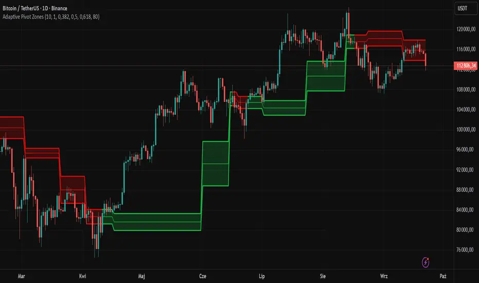
Adaptive Pivot Zones█ OVERVIEW
The "Adaptive Pivot Zones" indicator is a versatile tool designed to identify and visualize key pivot levels directly on the price chart. By detecting pivot highs and lows, the indicator calculates dynamic support and resistance zones based on user-defined levels (default: 0.382, 0.5, 0.618). These zones adapt to market volatility, providing traders with clear visual cues for potential reversal or continuation points. The indicator offers extensive customization options, such as adjusting colors, smoothing lines, and setting fill transparency, making it highly adaptable to various trading styles.
█ CONCEPTS
The "Adaptive Pivot Zones" indicator simplifies the identification of significant price levels by plotting three dynamic pivot lines, which can be smoothed to reduce market noise. The indicator dynamically changes the colors of the lines and fill zones based on price action, using bullish, bearish, or neutral colors to reflect market sentiment.
█ CALCULATIONS
The indicator relies on the following calculations:
- Pivot Detection: Pivot highs (ta.pivothigh) and pivot lows (ta.pivotlow) are identified using a user-defined pivot length (default: 10). Pivots represent significant price peaks and troughs. Higher pivot length values produce more stable levels but introduce a delay equal to the set value. For more aggressive strategies, the pivot length can be reduced.
- Pivot Levels: When both a pivot high and low are detected, the range between them is calculated (rng = drHigh - drLow). Three pivot levels are computed as:
Line 1: drLow + rng * pivotLevel1
Line 2: drLow + rng * pivotLevel2
Line 3: drLow + rng * pivotLevel3
- Smoothing: Pivot lines can be smoothed using a simple moving average (SMA) with a user-defined smoothing length (default: 1) to reduce noise and improve readability.
- Color Logic: Lines and fill zones are colored based on the price position relative to the pivot zones:
If the price is below the lowest pivot line, a bearish color is used (default: red).
If the price is above the highest pivot line, a bullish color is used (default: green).
If the price is within the pivot zones and the neutral color option is enabled, a neutral color is used (default: gray); otherwise, the previous color is retained.
- Fill Zones: The areas between pivot lines are filled with a user-defined transparency level (default: 80) to visually highlight support and resistance zones.
█ INDICATOR FEATURES
- Dynamic Pivot Lines: Three adaptive pivot lines (default levels: 0.382, 0.5, 0.618) are plotted on the price chart, adjusting to market volatility.
- Smoothing: User-defined smoothing length (default: 1) for pivot lines to reduce noise and enhance signal clarity.
- Dynamic Coloring: Lines and fill zones change color based on price action (bullish, bearish, or neutral when the price moves within the zone), reflecting market sentiment.
- Fill Zones: Transparent fills between pivot lines to visually highlight support and resistance zones.
- Customization: Options to adjust pivot length, pivot levels, smoothing, colors, transparency, and enable/disable neutral color logic.
█ HOW TO SET UP THE INDICATOR
- Add the "Adaptive Pivot Zones" indicator to your TradingView chart.
- Configure parameters in the settings, such as pivot length, pivot levels, smoothing length, and colors, to align with your trading strategy. Without smoothing, lines behave like levels; with smoothing, they act like bands. All three levels can be set to the same value to obtain a single level or a line behaving like a moving average derived from pivots.
- Enable or disable the neutral color option (for prices moving within the zone) and adjust fill transparency for optimal visualization.
- Adjust line thickness and style in the "Style" section to improve chart readability.
Example of bands – lines behave like support/resistance zones.
Example of a moving average derived from pivots – line behaves like a pivot-based MA.
█ HOW TO USE
Add the indicator to your chart, adjust the settings, and observe price interactions with the pivot lines and zones to identify potential trading opportunities. Key signals include:
- Price Interaction with Pivot Lines: When the price approaches or crosses a pivot line, it may indicate a potential support or resistance level. A bounce from a pivot line could signal a reversal, while a breakout might suggest trend continuation.
- Zone-Based Signals and Trend Line Usage: Price movement within or outside the filled zones can indicate market sentiment. Price below the lowest pivot line suggests bearish momentum, price above the highest pivot line suggests bullish momentum, and price within the zones may indicate consolidation. With higher pivot length values, the indicator can be used as a trend line, particularly during clear market movements.
- Color Changes: Shifts in line and fill colors (bullish, bearish, or neutral) provide visual cues about changing market conditions.
- Confirmation with Other Tools: Combine the indicator with tools like RSI or Bollinger Bands to validate signals and improve trade accuracy. For example, a buy signal from RSI in the oversold zone combined with a bounce from the lowest pivot line may indicate a strong entry point.
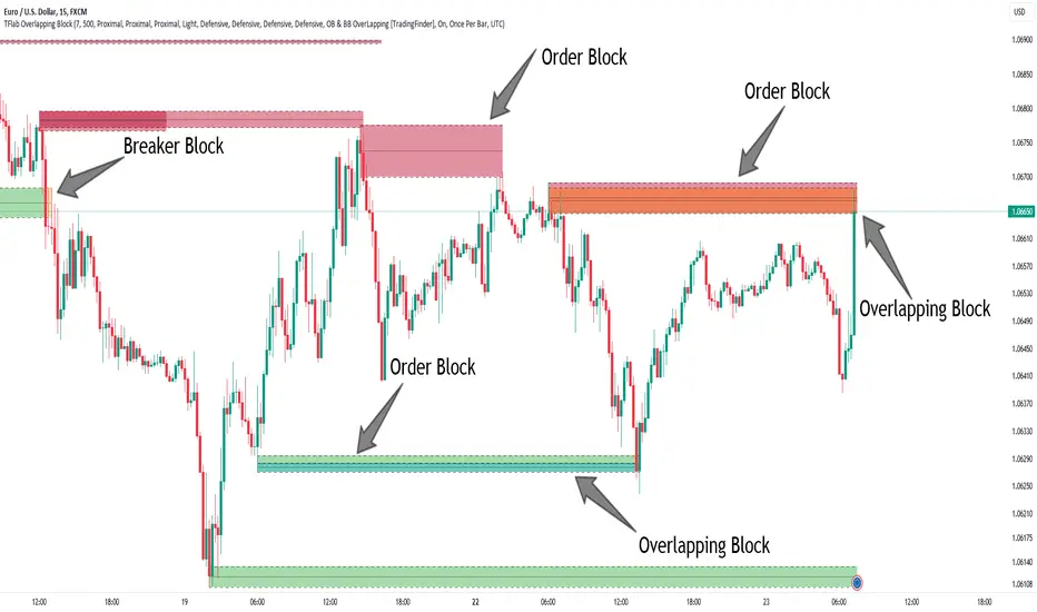
Breaker Blocks + Order Blocks confirm [TradingFinder] BBOB Alert🔵 Introduction
In the realm of technical analysis, various tools and concepts are employed to identify key levels on price charts. These tools assist traders in analyzing market trends with greater precision, enabling them to optimize their trading decisions. Among these tools, the Order Block and Breaker Block hold a significant place, serving as effective instruments for analyzing market structure.
🟣 Order Block
An Order Block refers to zones on a chart where large financial institutions and high-volume traders place their orders. Due to the substantial volume of buy or sell orders in these areas, they are often regarded as pivotal points for potential price reversals or temporary pauses in a trend. Order Blocks are particularly crucial when prices react to these zones after a strong market move, acting as strong support or resistance levels.
🟣 Breaker Block
On the other hand, a Breaker Block refers to areas on a chart that previously functioned as Order Blocks but where the price has managed to break through and continue in the opposite direction. These zones are typically recognized as key points where market trends might shift, helping traders identify potential reversal points in the market.
🟣 Overlapping Block (BBOB)
Now, imagine a scenario where these two essential concepts in technical analysis—Order Blocks and Breaker Blocks—overlap on a chart. Although this overlap is not specifically discussed within the ICT (Inner Circle Trader) trading framework, exploring and utilizing this overlap can provide traders with powerful insights into strong support and resistance zones. The combination of these two robust concepts can highlight critical areas in trading, potentially offering significant advantages in making informed trading decisions.
In this article, we will delve into the concept of this overlap, explaining how to utilize it in trading strategies. Additionally, we will analyze the potential outcomes and benefits of incorporating this concept into your trading decisions.
Bullish Overlapping Block (BBOB) :
Bearish Overlapping Block (BBOB) :
🔵 How to Use
The overlap between Order Blocks and Breaker Blocks is a compelling and powerful concept that can help traders identify key levels on the chart with a high probability of success. This overlap is particularly valuable because it combines two well-regarded concepts in technical analysis—zones of high order volume and critical market shifts.
🟣 Here’s how to effectively use this overlap in your trading
1. Dentifying the Overlapping Block : To make the most of the overlap between Order Blocks and Breaker Blocks, begin by identifying these zones separately. Order Blocks are areas where price typically reacts and reverses after a strong market move.
Breaker Blocks are areas where a previous Order Block has been breached, and the price continues in the opposite direction. When these two zones overlap on a chart, it’s crucial to pay close attention to this area, as it represents a high-probability reaction zone.
2. Analyzing the Overlapping Block : After identifying the overlap zone, carefully analyze price action within this region. Candlestick patterns and price behavior can provide essential clues.
If the price reaches this overlap zone and strong reversal patterns such as Pin Bars or Engulfing patterns are observed, it’s likely that this zone will act as a pivotal reversal point. In such cases, entering a trade with confidence becomes more feasible.
3. Entering the Trade : When sufficient signs of price reaction are present in the overlap zone, you can proceed to enter the trade. If the overlap zone is within an uptrend and bullish reversal signals are evident, a long position might be appropriate.
Conversely, if the overlap zone is in a downtrend and bearish reversal signals are observed, a short position would be more suitable.
4. Risk Management : One of the most critical aspects of trading in overlap zones is managing risk. To protect your capital, place your stop loss near the lowest point of the Order Block (for buy trades) or the highest point (for sell trades). This approach minimizes potential losses if the overlap zone fails to hold.
5. Price Targets : After entering the trade, set your price targets based on other key levels on the chart. These targets could include other support and resistance zones, Fibonacci levels, or pivot points.
Bullish Overlapping Block :
Bearish Overlapping Block :
🟣 Benefits of the Overlapping Block Between Order Block and Breaker Block
1. Enhanced Precision in Identifying Key Levels : The overlap between these two zones usually acts as a highly reliable area for price reactions, increasing the accuracy of identifying entry and exit points.
2. Reduced Trading Risk : Given the high importance of the overlap zone, the likelihood of making incorrect decisions is reduced, contributing to overall lower trading risk.
3. Increased Probability of Success : The overlap between Order Blocks and Breaker Blocks combines two powerful concepts, enhancing the likelihood of success in trades, as multiple indicators confirm the importance of the area.
4. Creation of Better Trading Opportunities : Overlap zones often provide traders with more robust trading opportunities, as these areas typically represent strong reversal points in the market.
5. Compatibility with Other Technical Tools : This concept seamlessly integrates with other technical analysis tools such as Fibonacci retracements, trend lines, and chart patterns, offering a more comprehensive market analysis.
🔵 Setting
🟣 Global Setting
Pivot Period of Order Blocks Detector : Enter the desired pivot period to identify the Order Block.
Order Block Validity Period (Bar) : You can specify the maximum time the Order Block remains valid based on the number of candles from the origin.
Mitigation Level Order Block : Determining the basic level of a Order Block. When the price hits the basic level, the Order Block due to mitigation.
Mitigation Level Breaker Block : Determining the basic level of a Breaker Block. When the price hits the basic level, the Breaker Block due to mitigation.
Mitigation Level Overlapping Block : Determining the basic level of a Overlapping Block. When the price hits the basic level, the Overlapping Block due to mitigation.
🟣 Overlapping Block Display
Show All Overlapping Block : If it is turned off, only the last Order Block will be displayed.
Demand Overlapping Block : Show or not show and specify color.
Supply Overlapping Block : Show or not show and specify color.
🟣 Order Block Display
Show All Order Block : If it is turned off, only the last Order Block will be displayed.
Demand Main Order Block : Show or not show and specify color.
Demand Sub (Propulsion & BoS Origin) Order Block : Show or not show and specify color.
Supply Main Order Block : Show or not show and specify color.
Supply Sub (Propulsion & BoS Origin) Order Block : Show or not show and specify color.
🟣 Breaker Block Display
Show All Breaker Block : If it is turned off, only the last Breaker Block will be displayed.
Demand Main Breaker Block : Show or not show and specify color.
Demand Sub (Propulsion & BoS Origin) Breaker Block : Show or not show and specify color.
Supply Main Breaker Block : Show or not show and specify color.
Supply Sub (Propulsion & BoS Origin) Breaker Block : Show or not show and specify color.
🟣 Order Block Refinement
Refine Order Blocks : Enable or disable the refinement feature. Mode selection.
🟣 Alert
Alert Name : The name of the alert you receive.
Alert Overlapping Block Mitigation :
On / Off
Message Frequency :
This string parameter defines the announcement frequency. Choices include: "All" (activates the alert every time the function is called), "Once Per Bar" (activates the alert only on the first call within the bar), and "Once Per Bar Close" (the alert is activated only by a call at the last script execution of the real-time bar upon closing). The default setting is "Once per Bar".
Show Alert Time by Time Zone :
The date, hour, and minute you receive in alert messages can be based on any time zone you choose. For example, if you want New York time, you should enter "UTC-4". This input is set to the time zone "UTC" by default.
🔵 Conclusion
The overlap between Order Blocks and Breaker Blocks represents a critical and powerful area in technical analysis that can serve as an effective tool for determining entry and exit points in trading.
These zones, due to the combination of two key concepts in technical analysis, hold significant importance and can help traders make more confident trading decisions.
Although this concept is not specifically discussed in the ICT framework and is introduced as a new idea, traders can achieve better results in their trades through practice and testing.
Utilizing the overlap between Order Blocks and Breaker Blocks, in conjunction with other technical analysis tools, can significantly improve the chances of success in trading.
Best Buying & Selling Flip Zone @MaxMaserati 3.0Best Buying & Selling Flip Zone 3.0 🐂🐻
Best Buying & Selling Flip Zone 3.0 is an advanced, multi-timeframe Price Action tool designed to identify high-probability institutional supply and demand zones.
By analyzing candle range and body size (Expander vs. Normal candles), this indicator categorizes market structure shifts into three distinct tiers of strength (A+++, A++, A+). It includes a built-in Trade Manager, Volume Tracking, and a unique "Defender/Attacker" Multi-Timeframe (MTF) entry confirmation system.
🚀 Key Features
Multi-Timeframe Analysis: Monitor Higher Timeframe (HTF) zones while trading on a Lower Timeframe (LTF).
Tiered Setup Grading: Automatically classifies zones based on the strength of the candle engulfing action (King Slayer, Crusher, Drift).
Smart Entry Confirmation: The script can wait for price to tap an HTF zone and then automatically search for a confirmation pattern on the current timeframe before signaling a trade.
Built-in Trade Management: Visualizes Entry, Stop Loss (SL), and Take Profit (TP) levels with customizable Risk:Reward ratios.
Volume Tracking: Monitors the volume utilized to create a zone and tracks "remaining" volume as price tests the zone.
Zone Deletion Logic: Automatically removes zones that have been invalidated by either a wick or a candle close.
🧠 How It Works: The "A-Grade" Logic
The indicator analyzes candles based on their body-to-range ratio to define "Expander" (Explosive move) vs. "Normal" candles. It then looks for engulfing behaviors to create zones:
A+++ (King Slayer):
Logic: A Bullish Expander engulfs a Bearish Expander (or vice versa).
Significance: This is the strongest signal, indicating a massive shift in momentum where aggressive buyers completely overwhelmed aggressive sellers.
A++ (Crusher):
Logic: A Bullish Expander engulfs a Bearish Normal candle.
Significance: Strong momentum overcoming standard price action. High probability.
A+ (Drift):
Logic: A Bullish Normal candle engulfs a Bearish Normal candle.
Significance: A standard flip zone. Good for continuation plays but less aggressive than KS or CR setups.
🛠️ Functionality Guide
1. General Filters & Timeframes
Higher Timeframe: Select a timeframe higher than your chart (e.g., Select 4H while trading on 15m). The indicator will draw the major zones from the 4H.
Deletion Logic:
Wick (Hard): Zone is removed immediately if price touches the invalidation level.
Close (Soft): Zone is removed only if a candle closes past the invalidation level.
2. LTF Entry Confirmation (The "Master" Switch)
When Show LTF Entry Logic is enabled, the indicator does not signal immediately upon an HTF zone creation. Instead:
It waits for the price to retraced and touch the HTF zone.
Once touched, it scans the current timeframe for a valid flip setup (KS, CR, or DR).
It creates a tighter entry box and draws trade lines only when this confirmation occurs.
3. Trade Management
Risk:Reward: Set your desired RR (e.g., 2.0).
SL Padding: Add breathing room (ticks) to your Stop Loss.
SL Source: Choose between a safer Stop Loss (based on the HTF zone) or a tighter Stop Loss (based on the LTF confirmation candle).
4. Volume Stats
Labels display the volume involved in the zone's creation. As price taps the zone, the volume is "depleted" from the label, giving you insight into the remaining order flow absorption.
🎨 Visual Customization
Colors: Fully customizable colors for Buyers (Green) and Sellers (Red) zones across all three strength tiers.
Labels: Toggle technical names, touch counts, and timeframe labels.
Lines: Option to show "Aggressive Open Lines" to mark the exact opening price of the flip zone extended forward.
⚠️ Disclaimer
This tool is for educational purposes and chart analysis assistance only. Past performance of a setup (A+++/King Slayer) does not guarantee future results. Always manage risk and use this in conjunction with your own trading strategy.

Smart Money Zones (FVG + OB) + MTF Trend Panel## Overview
Professional-grade institutional trading zones indicator that identifies **Fair Value Gaps (FVG)** and **Order Blocks (OB)** - key price inefficiencies where smart money operates. Includes a comprehensive **Multi-Timeframe Trend Panel** for complete market context at a glance.
## Core Features
### 🎯 Fair Value Gaps (FVG)
Fair Value Gaps occur when price moves so aggressively that it leaves an "imbalance" or "gap" in the market structure. These zones often act as magnets where price returns to find liquidity.
**Detection Logic:**
- **Bullish FVG**: When current candle's low is above the high of the candle 2 bars ago
- **Bearish FVG**: When current candle's high is below the low of the candle 2 bars ago
- Requires strong impulse candle (configurable body percentage threshold)
- Color-coded zones: Green for bullish, Red for bearish
### 📦 Order Blocks (OB)
Order Blocks represent the last opposite candle before a significant price move - the zone where institutional orders were placed before the breakout.
**Detection Logic:**
- Identifies the last bearish candle before a strong bullish breakout (Bullish OB)
- Identifies the last bullish candle before a strong bearish breakout (Bearish OB)
- Validates breakout strength using ATR multiplier (1.2x default)
- Color-coded zones: Blue for bullish, Orange for bearish
### 📊 Multi-Timeframe Trend Panel
Real-time trend analysis across **7 timeframes** displayed in an elegant dashboard:
- **1 Minute** - Ultra short-term scalping
- **5 Minutes** - Short-term momentum
- **15 Minutes** - Intraday swings
- **30 Minutes** - Session trends
- **1 Hour** - Multi-session trends
- **4 Hours** - Daily structure
- **Daily** - Long-term direction
**Visual Indicators:**
- 🟢 Green circle = Bullish trend
- 🔴 Red circle = Bearish trend
- Clean, professional table design with customizable position and size
## Intelligence Features
### 🧠 Zone Strength Rating
Every zone is automatically classified by strength based on size relative to ATR:
- **VERY STRONG** - 2.0x ATR or more (major institutional zones)
- **STRONG** - 1.5x to 2.0x ATR (significant zones)
- **MEDIUM** - 1.0x to 1.5x ATR (moderate zones)
- **WEAK** - Below 1.0x ATR (minor zones)
Strength rating helps you prioritize which zones to trade from!
### 📉 Smart Mitigation Tracking
Zones automatically track how much they've been "filled" or mitigated:
- Calculates penetration percentage as price enters the zone
- Zones turn **gray** when 50%+ mitigated or fully filled
- Option to **auto-delete** mitigated zones to keep chart clean
- Live zones extend dynamically with price action
### 🎨 Trend Filter (Optional)
When enabled, only shows zones aligned with the current trend:
- Uses customizable MA period (default 50)
- Bullish zones only appear in uptrend
- Bearish zones only appear in downtrend
- Reduces noise and false signals significantly
## Customization Options
### Display Settings
- Toggle FVGs and OBs independently
- Adjust max zones per type (5-200)
- Choose to remove or gray out mitigated zones
- Color customization for all zone types
### Detection Parameters
- **Min Impulse Body %**: Controls how strong the impulse candle must be (0.3-1.0)
- **Order Block Lookback**: How many bars to look back for OB validation (5-50)
- **ATR Length**: Period for ATR calculation (5-50)
### Trend Filter
- Enable/disable trend filtering
- Adjustable MA period for trend determination
### MTF Panel
- Show/hide the trend panel
- 4 position options: Top Right, Top Left, Bottom Right, Bottom Left
- 3 size options: Small, Normal, Large
- Customizable MA period for trend calculation across all timeframes
## Trading Applications
### 1. **Liquidity Grab Entries**
Wait for price to sweep a zone (50%+ mitigation) then enter on reversal. Smart money often "hunts" these zones before the real move begins.
### 2. **Confluence Trading**
Look for zones that align with:
- Multiple timeframe trends showing same direction
- Multiple FVGs/OBs stacking in same area
- Key support/resistance levels
### 3. **Breakout Confirmation**
Use Order Blocks to confirm the strength of breakouts. Strong OBs indicate institutional participation.
### 4. **Retracement Entries**
Enter when price returns to a fresh, unmitigated zone in the direction of the higher timeframe trend.
### 5. **Range Trading**
Identify FVG zones at range extremes - price often reverses at these inefficiencies.
## How It Works
**Fair Value Gaps** form when the middle candle creates such aggressive movement that it leaves a price gap between the high/low of surrounding candles. Institutional traders know these gaps get filled.
**Order Blocks** mark the origin of major moves. The last opposite-colored candle before a breakout is where large orders were placed. Price often returns to these zones for "retests" before continuing.
**Mitigation** happens when price returns to fill these zones. The indicator tracks this automatically, showing you which zones are still "fresh" and which have been used up.
## Best Practices
✅ **Use higher timeframe trends** - Always check the MTF panel before taking trades
✅ **Trade fresh zones** - Unmitigated zones (not gray) have the highest probability
✅ **Combine with price action** - Look for rejection wicks and engulfing candles at zones
✅ **Respect zone strength** - VERY STRONG and STRONG zones are most reliable
✅ **Use trend filter** - Especially on lower timeframes to reduce false signals
❌ **Don't overtrade** - Not every zone will react, wait for confirmation
❌ **Don't ignore context** - Check the MTF panel for conflicting trends
❌ **Don't chase** - Wait for price to come to the zone, don't enter mid-zone
## Technical Details
- **Non-repainting**: All zones are drawn on confirmed candles only
- **Performance optimized**: Uses efficient array management with per-type caps
- **Real-time updates**: Zones extend and track mitigation as price moves
- **Universal compatibility**: Works on all markets and timeframes
## Recommended Settings by Style
**Scalping (1m-5m charts):**
- Max zones: 10-15
- Use trend filter: ON
- MTF Panel: Focus on 1m-15m trends
- Remove mitigated: ON (keep chart clean)
**Day Trading (5m-1H charts):**
- Max zones: 15-20
- Use trend filter: ON
- MTF Panel: Focus on 15m-4H trends
- Remove mitigated: OFF (track zone history)
**Swing Trading (1H-D charts):**
- Max zones: 20+
- Use trend filter: Optional
- MTF Panel: Focus on 1H-1D trends
- Remove mitigated: OFF (important zones persist)
---
## Perfect For
- Smart Money Concept (SMC) traders
- ICT methodology followers
- Institutional order flow traders
- Price action traders seeking key zones
- Multi-timeframe analysis enthusiasts
**Compatible with all markets:** Forex, Crypto, Stocks, Indices, Commodities, Futures
*Trade where the institutions trade. Follow the smart money.*

Time-Decay Liquidity Zones [BackQuant]Time-Decay Liquidity Zones
A dynamic liquidity map that turns single-bar exhaustion events into fading, color-graded zones, so you can see where trapped traders and unfinished business still matter, and when those areas have finally stopped pulling price.
What this is
This indicator detects unusually strong impulsive moves into wicks, converts them into supply or demand “zones,” then lets those zones decay over time. Each zone carries a strength score that fades bar by bar. Zones that stop attracting or rejecting price are gradually de-emphasized and eventually removed, while the most relevant areas stay bright and obvious.
Instead of static rectangles that live forever, you get a living liquidity map where:
Zones are born from objective criteria: volatility, wick size, and optional volume spikes.
Zones “age” using a configurable decay factor and maximum lifetime.
Zone color and opacity reflect current relative strength on a unified clear → green → red gradient.
Zones freeze when broken, so you can distinguish “active reaction areas” from “historical levels that have already given way”.
Conceptual idea
Large wicks with strong volatility often mark areas where aggressive orders met hidden liquidity and got absorbed. Price may revisit these areas to test leftover interest or to relieve trapped positions. However, not every wick matters for long. As time passes and more bars print, the market “forgets” some areas.
Time-Decay Liquidity Zones turns that idea into a rule-based system:
Find bars that likely reflect strong aggressive flows into liquidity.
Mark a zone around the wick using ATR-based thickness.
Assign a strength score of 1.0 at birth.
Each bar, reduce that score by a decay factor and remove zones that fall below a threshold or live too long.
Color all surviving zones from weak to strong using a single gradient scale and a visual legend.
How events are detected
Detection lives in the Event Detection group. The script combines range, wick size, and optional volume filters into simple rules.
Volatility filter
ATR Length — computes a rolling ATR over your chosen window. This is the volatility baseline.
Min range in ATRs — bar range (High–Low) must exceed this multiple of ATR for an event to be considered. This avoids tiny bars triggering zones.
Wick filters
For each bar, the script splits the candle into body and wicks:
Upper wick = High minus the max(Open, Close).
Lower wick = min(Open, Close) minus Low.
Then it tests:
Upper wick condition — upper wick must be larger than Min wick size in ATRs × ATR.
Lower wick condition — lower wick must be larger than Min wick size in ATRs × ATR.
Only bars with a sufficiently long wick relative to volatility qualify as candidate “liquidity events”.
Volume filter
Optionally, the script requires a volume spike:
Use volume filter — if enabled, volume must exceed a rolling volume SMA by a configurable multiplier.
Volume SMA length — period for the volume average.
Volume spike multiplier — how many times above the SMA current volume needs to be.
This lets you focus only on “heavy” tests of liquidity and ignore quiet bars.
Event types
Putting it together:
Upper event (potential supply / long liquidation, etc.)
Occurs when:
Upper wick is large in ATR terms.
Full bar range is large in ATR terms.
Volume is above the spike threshold (if enabled).
Lower event (potential demand / short liquidation, etc.)
Symmetric conditions using the lower wick.
How zones are constructed
Zone geometry lives in Zone Geometry .
When an event is detected, the script builds a rectangular box that anchors to the wick and extends in the appropriate direction by an ATR-based thickness.
For upper (supply-type) zones
Bottom of the zone = event bar high.
Top of the zone = event bar high + Zone thickness in ATRs × ATR.
The zone initially spans only the event bar on the x-axis, but is extended to the right as new bars appear while the zone is active.
For lower (demand-type) zones
Top of the zone = event bar low.
Bottom of the zone = event bar low − Zone thickness in ATRs × ATR.
Same extension logic: box starts on the event bar and grows rightward while alive.
The result is a band around the wick that scales with volatility. On high-ATR charts, zones are thicker. On calm charts, they are narrower and more precise.
Zone lifecycle, decay, and removal
All lifecycle logic is controlled by the Decay & Lifetime group.
Each zone carries:
Score — a floating-point “importance” measure, starting at 1.0 when created.
Direction — +1 for upper zones, −1 for lower zones.
Birth index — bar index at creation time.
Active flag — whether the zone is still considered unbroken and extendable.
1) Active vs broken
Each confirmed bar, the script checks:
For an upper zone , the zone is counted as “broken” when the close moves above the top of the zone.
For a lower zone , the zone is counted as “broken” when the close moves below the bottom of the zone.
When a zone breaks:
Its right edge is frozen at the previous bar (no further extension).
The zone remains on the chart, but is no longer updated by price interaction. It still decays in score until removal.
This lets you see where a major level was overrun, while naturally fading its influence over time.
2) Time decay
At each confirmed bar:
Score := Score × Score decay per bar .
A decay value close to 1.0 means very slow decay and long-lived zones.
Lower values (closer to 0.9) mean faster forgetting and more current-focused zones.
You are controlling how quickly the market “forgets” past events.
3) Age and score-based removal
Zones are removed when either:
Age in bars exceeds Max bars a zone can live .
This is a hard lifetime cap.
Score falls below Minimum score before removal .
This trims zones that have decayed into irrelevance even if their age is still within bounds.
When a zone is removed, its box is deleted and all associated state is freed to keep performance and visuals clean.
Unified gradient and color logic
Color control lives in Gradient & Color . The indicator uses a single continuous gradient for all zones, above and below price, so you can read strength at a glance without guessing what palette means what.
Base colors
You set:
Mid strength color (green) — used for mid-level strength zones and as the “anchor” in the gradient.
High strength color (red) — used for the strongest zones.
Max opacity — the maximum visual opacity for the solid part of the gradient. Lower values here mean more solid; higher values mean more transparent.
The script then defines three internal points:
Clear end — same as mid color, but with a high alpha (close to transparent).
Mid end — mid color at the strongest allowed opacity.
High end — high color at the strongest allowed opacity.
Strength normalization
Within each update:
The script finds the maximum score among all existing zones.
Each zone’s strength is computed as its score divided by this maximum.
Strength is clamped into .
This means a zone with strength 1.0 is currently the strongest zone on the chart. Other zones are colored relative to that.
Piecewise gradient
Color is assigned in two stages:
For strength between 0.0 and 0.5: interpolate from “clear” green to solid green.
Weak zones are barely visible, mid-strength zones appear as solid green.
For strength between 0.5 and 1.0: interpolate from solid green to solid red.
The strongest zones shift toward the red anchor, clearly separating them from everything else.
Strength scale legend
To make the gradient readable, the indicator draws a vertical legend on the right side of the chart:
About 15 cells from top (Strong) to bottom (Weak).
Each cell uses the same gradient function as the zones themselves.
Top cell is labeled “Strong”; bottom cell is labeled “Weak”.
This legend acts as a fixed reference so you can instantly map a zone’s color to its approximate strength rank.
What it plots
At a glance, the indicator produces:
Upper liquidity zones above price, built from large upper wick events.
Lower liquidity zones below price, built from large lower wick events.
All zones colored by relative strength using the same gradient.
Zones that freeze when price breaks them, then fade out via decay and removal.
A strength scale legend on the right to interpret the gradient.
There are no extra lines, labels, or clutter. The focus is the evolving structure of liquidity zones and their visual strength.
How to read the zones
Bright red / bright green zones
These are your current “major” liquidity areas. They have high scores relative to other zones and have not yet decayed. Expect meaningful reactions, absorption attempts, or spillover moves when price interacts with them.
Faded zones
Pale, nearly transparent zones are either old, decayed, or minor. They can still matter, but priority is lower. If these are in the middle of a long consolidation, they often become background noise.
Broken but still visible zones
Zones whose extension has stopped have been overrun by closing price. They show where a key level gave way. You can use them as context for regime shifts or failed attempts.
Absence of zones
A chart with few or no zones means that, under your current thresholds, there have not been strong enough liquidity events recently. Either tighten the filters or accept that recent price action has been relatively balanced.
Use cases
1) Intraday liquidity hunting
Run the indicator on lower timeframes (e.g., 1–15 minute) with moderately fast decay.
Use the upper zones as potential sell reaction areas, the lower zones as potential buy reaction areas.
Combine with order flow, CVD, or footprint tools to see whether price is absorbing or rejecting at each zone.
2) Swing trading context
Increase ATR length and range/wick multipliers to focus only on major spikes.
Set slower decay and higher max lifetime so zones persist across multiple sessions.
Use these zones as swing inflection areas for larger setups, for example anticipating re-tests after breakouts.
3) Stop placement and invalidation
For longs, place invalidation beyond a decaying lower zone rather than in the middle of noise.
For shorts, place invalidation beyond strong upper zones.
If price closes through a strong zone and it freezes, treat that as additional evidence your prior bias may be wrong.
4) Identifying trapped flows
Upper zones formed after violent spikes up that quickly fail can mark trapped longs.
Lower zones formed after violent spikes down that quickly reverse can mark trapped shorts.
Watching how price behaves on the next touch of those zones can hint at whether those participants are being rescued or squeezed.
Settings overview
Event Detection
Use volume filter — enable or disable the volume spike requirement.
Volume SMA length — rolling window for average volume.
Volume spike multiplier — how aggressive the volume spike filter is.
ATR length — period for ATR, used in all size comparisons.
Min wick size in ATRs — minimum wick size threshold.
Min range in ATRs — minimum bar range threshold.
Zone Geometry
Zone thickness in ATRs — vertical size of each liquidity zone, scaled by ATR.
Decay & Lifetime
Score decay per bar — multiplicative decay factor for each zone score per bar.
Max bars a zone can live — hard cap on lifetime.
Minimum score before removal — score cut-off at which zones are deleted.
Gradient & Color
Mid strength color (green) — base color for mid-level zones and the lower half of the gradient.
High strength color (red) — target color for the strongest zones.
Max opacity — controls the most solid end of the gradient (0 = fully solid, 100 = fully invisible).
Tuning guidance
Fast, session-only liquidity
Shorter ATR length (e.g., 20–50).
Higher wick and range multipliers to focus only on extreme events.
Decay per bar closer to 0.95–0.98 and moderate max lifetime.
Volume filter enabled with a decent multiplier (e.g., 1.5–2.0).
Slow, structural zones
Longer ATR length (e.g., 100+).
Moderate wick and range thresholds.
Decay per bar very close to 1.0 for slow fading.
Higher max lifetime and slightly higher min score threshold so only very weak zones disappear.
Noisy, high-volatility instruments
Increase wick and range ATR multipliers to avoid over-triggering.
Consider enabling the volume filter with stronger settings.
Keep decay moderate to avoid the chart getting overloaded with old zones.
Notes
This is a structural and contextual tool, not a complete trading system. It does not account for transaction costs, execution slippage, or your specific strategy rules. Use it to:
Highlight where liquidity has recently been tested hard.
Rank these areas by decaying strength.
Guide your attention when layering in separate entry signals, risk management, and higher-timeframe context.
Time-Decay Liquidity Zones is designed to keep your chart focused on where the market has most recently “cared” about price, and to gradually forget what no longer matters. Adjust the detection, geometry, decay, and gradient to fit your product and timeframe, and let the zones show you which parts of the tape still have unfinished business.

Thrax - Intraday Market Pressure ZonesTHRAX - INTRADAY MARKET PRESSURE ZONES
This indicator identifies potential support and resistance zones based on areas of significant market pressure. It dynamically plots these zones and adjusts their visibility based on real-time price action and user-defined thresholds. The indicator is useful for traders seeking to understand intraday market pressure, visualize zones of potential price reversals, and analyze volume imbalances at critical levels.
1. Support/Resistance Zones: Wherever the price retraces significantly from its high a support zone is drawn and when it retraces significantly from it low a resistance zone is drawn. The significant retracing is measured by the wick threshold percentage. For instance, if set to 75%, it implies price retracement of 75% either from high or from low for a particular candel
Volume delat: Displays volume delta information where the zones are formed. This can be used by trader to consider only those zones where delta is significant.
2. Breakout Detection: Monitors for price breakouts beyond established zones, deleting zones that are invalidated by price movement. when the price breaks a given zone with the threshold, it is considered to be mitigated and chances of trend continuation is decent.
Candle Coloring: Uses color codes (green, red, and yellow) to represent bullish, bearish, and indecisive (doji) candles, aiding quick visual assessment.
INPUTS
1. Wick Threshold (%) : Sets the minimum wick percentage required for a candle to be considered a support or resistance candidate.
2. Breakout Threshold (%) : Determines the percentage above or below a support or resistance zone that defines a breakout condition. if breaks a zone with the set threshold then the zone will be considered mititgated.
3. Max Number of Support/Resistance Zones : Limits the maximum number of support/resistance zones displayed on the chart, ranging from 1 to 5.
4. Show Wick Percentage Labels : Toggles the display of percentage values for upper and lower wicks on each candle.
TRADE SETUP
Identifying Entry Points: Look for the formation of support or resistance zones. Wait for price to retrace to these zones. if you are willing to take risk, you can consider even zones with low delta. If you want to be more cautious you should consider zones with high delta.
Volume Confirmation: Use the volume information to confirm the strength of the zone. Strong volume differences (displayed as labels) can indicate significant market pressure at these levels.
Breakout Trades: If price breaks through a support/resistance zone by more than the breakout threshold, consider this a signal for a potential trend continuation in the breakout direction.
Risk Management: Set stop-loss levels slightly outside of the identified zones to minimize risk in case of false breakouts. This can be set in input setting for breakout threshold.
Bonus Tip : Mark your significant highs and lows from where prices have retraced multiple times in the near past and if the zone is near these levels it can serve s a strong candidate of support or resistance
Therefore, in conclusion monitor the zones, based on delta and volume presence filter out the zone, wait for price retracement to the zone, intiate the trade with stop loss below zone with a set percentage.
Liquidity Zones [BigBeluga]This indicator is designed to detect liquidity zones on the chart by identifying significant pivot highs and lows filtered by volume strength. It plots these zones as boxes, highlighting areas where liquidity is likely to accumulate. The indicator also draws lines extending from these boxes, marking the levels where price may "grab" this liquidity. The size of these boxes can be dynamic, adjusting based on the volume size, offering a visual representation of market areas where traders might expect significant price reactions.
🔵 IDEA
The idea behind the Liquidity Zones indicator is to help traders identify key market levels where liquidity accumulates. Liquidity zones are areas where there are enough buy or sell orders that can potentially lead to significant price movements. By focusing on pivot points filtered by volume strength, the indicator aims to provide a clearer picture of where large players may have positioned their orders. This insight allows traders to anticipate potential market reactions, such as reversals or breakouts, when the price reaches these zones. The option for dynamic box height further refines the visualization, showing the extent of liquidity based on the volume's intensity.
🔵 KEY FEATURES & USAGE
◉ Volume-Filtered Pivot Highs and Lows:
The indicator scans for pivot highs and lows on the chart, filtering these points based on the volume strength setting (Low, Mid, High). This ensures that only the most significant liquidity zones, backed by notable trading volume, are highlighted. Traders can adjust the filter to focus on different levels of market activity, from small fluctuations to major volume spikes.
Low:
Mid:
High:
◉ Dynamic and Static Liquidity Zones:
Liquidity zones are plotted as boxes around pivot points, with an optional dynamic mode that adjusts the box height based on the normalized volume. This dynamic adjustment reflects the liquidity carried by the volume, making it easier to gauge the significance of each zone. In static mode, the boxes have a fixed height, providing a consistent visual reference for the zones.
◉ Color Intensity Based on Volume:
The indicator adjusts the color intensity of the liquidity zones based on the volume strength. Higher volume zones will be displayed with more intense colors, giving a visual cue to the strength of the liquidity present in that area. This makes it easier to differentiate between zones of varying importance at a glance, allowing traders to quickly identify where the market has the highest concentration of liquidity.
◉ Liquidity Grab Detection and Red Circles:
When the price interacts with a liquidity zone, the indicator detects whether liquidity has been "grabbed" at these levels. If the price moves into a zone and crosses a level, the box label changes to "Liquidity Grabbed," and the line marking the level becomes dashed.
Reversal Points:
The beginning of a trend:
Additionally marks these "liquidity grabs" with red circles, indicating both recent and past liquidity grabs. This feature helps traders identify areas where liquidity has been absorbed by the market, which may signal potential reversals or shifts in market direction.
◉ Dashboard Display:
A dashboard in the upper right corner of the chart provides an overview of the indicator's settings and status. It shows the number of plotted zones, as set in the input settings, and whether the dynamic mode is active. This quick reference helps traders stay informed about the indicator's configuration without needing to open the settings panel.
🔵 CUSTOMIZATION
Length & Zones Amount: Set the length for pivot detection and the maximum number of zones to be displayed on the chart. This allows you to control how many liquidity zones you want to monitor at any given time.
Volume Strength Filter: Adjust the filter to Low, Mid, or High to control the strength of volume required for a pivot to be considered a significant liquidity zone. Higher settings focus on zones with greater volume, indicating stronger liquidity.
Dynamic Distance Mode: Enable or disable the dynamic mode, which adjusts the box height based on the volume size. When dynamic mode is off, the boxes have a fixed height based on the ATR, offering a consistent visualization regardless of the volume size.
The Liquidity Zones indicator is a versatile tool for identifying areas of significant market activity, offering a clear view of where liquidity is likely to reside. By filtering these zones through volume strength and providing dynamic or static visualization options, it equips traders with insights into potential market reaction points, enhancing their ability to anticipate and respond to market movements. The varying color intensity based on volume further aids in quickly recognizing the most critical liquidity zones on the chart.

ApEn Zones with Delta Confirmation MTF [PhenLabs]📊 ApEn Zones with Delta Confirmation MTF
Version: PineScript™ v6
📌 Description
The ApEn Zones with Delta Confirmation MTF indicator combines Approximate Entropy analysis with cumulative volume delta to identify high-probability support and resistance zones. Approximate Entropy (ApEn) measures the complexity and unpredictability in price data—when ApEn drops significantly, it signals a transition from chaotic to ordered market behavior, often preceding reversals or continuations.
This indicator goes beyond simple ApEn detection by integrating Delta confirmation, which validates zones using volume-based order flow analysis. When a zone forms with Delta confirmation, it indicates institutional participation aligning with the price structure. The multi-timeframe capability allows traders to detect zones forming on higher timeframes while executing on their preferred chart.
🚀 Points of Innovation
First indicator to combine ApEn complexity analysis with cumulative Delta confirmation for zone validation
Pre-built calculation presets eliminate guesswork—optimized parameters for scalping, day trading, and swing trading
Smart zone management automatically removes invalidated zones after two price rejections
Multi-timeframe architecture detects zones on configurable timeframes independent of chart timeframe
Visual style presets provide instant customization from high contrast to subtle overlays
Delta threshold system distinguishes between regular zones and institutionally-confirmed zones
🔧 Core Components
ApEn Calculator: Measures pattern regularity using embedding dimension (m=2) and tolerance factor (r) against price standard deviation to quantify market complexity
Delta Engine: Computes cumulative delta from volume and price movement, comparing against statistical thresholds to identify significant order flow divergence
Zone Generator: Creates visual box zones at signal points with dynamic sizing based on bar range and confirmation status
MTF Request Handler: Fetches ApEn calculations from user-specified timeframe using security() calls for higher timeframe alignment
Zone Manager: Tracks zone interactions, counts rejections, and automatically purges zones that have been tested twice
🔥 Key Features
Calculation Presets: Choose from Aggressive, Conservative, Scalping 1m, Strong Scalping, Swing Trading, or Default—each preset optimizes all parameters for specific trading styles
Visual Style Presets: Select Default, High Contrast, Subtle, Classic, Neutral, or Neutral Reverse to match your chart theme and preference
Delta Confirmation: Zones display with enhanced opacity when cumulative delta confirms institutional participation in the direction of the zone
Automatic Zone Cleanup: Zones self-destruct after two rejections, keeping your chart clean and focused on active levels
Alert System: Four alert conditions for buy zones, sell zones, strong buy signals, and strong sell signals
Maximum Zone Control: Limits display to 5 zones per direction to prevent chart clutter
🎨 Visualization
Buy Zones: Displayed as horizontal boxes at low points when ApEn crosses under threshold—lighter transparency indicates regular zone, darker indicates Delta confirmation
Sell Zones: Displayed as horizontal boxes at high points when ApEn crosses over threshold—visual confirmation follows same transparency logic
Zone Boundaries: Each zone extends 10% of bar range above and below the signal level, providing clear entry and stop areas
Dynamic Extension: All zones automatically extend rightward with each new bar until invalidated
📖 Usage Guidelines
Calculation Preset Selection
Scalping 1m / Strong Scalping: Use for 1-5 minute charts with faster signal generation and tighter thresholds (Length: 15, Zone Length: 5)
Aggressive: Shorter lookback (Length: 10) generates more zones with lower confirmation requirements—higher frequency, more noise
Default: Balanced parameters suitable for 5-15 minute charts (Length: 15, Zone Threshold: 0.5, Delta Length: 4)
Conservative: Extended lookback (Length: 30) with stricter thresholds—fewer but higher probability zones
Swing Trading: Longest parameters (Length: 40, Zone Length: 20) for 1H-4H charts capturing major structural zones
Visual Style Selection
High Contrast: Bright green/red for maximum visibility on any background
Subtle: Muted green/red with transparency for minimal chart distraction
Classic: Traditional lime green and crimson color scheme
Neutral / Neutral Reverse: Grayscale tones for non-directional bias visualization
Timeframe Configuration
Default timeframe is set to 1 minute—adjust based on your execution timeframe
For scalping: Set zone timeframe 1-3x your chart timeframe
For swing trading: Set zone timeframe to 4H or Daily while viewing 1H charts
✅ Best Use Cases
Identifying reversal zones during high-volatility market conditions
Confirming support/resistance levels with volume-based order flow validation
Scalping entries on lower timeframes with higher timeframe zone confluence
Filtering trade setups by requiring Delta confirmation before entry
Setting stop losses beyond zone boundaries after rejection tests
Swing trade positioning at zones detected on 4H/Daily timeframes
⚠️ Limitations
ApEn calculations are computationally intensive—may experience slower loading on very long chart histories
Delta estimation uses (close - open) * volume approximation, not actual order flow data
Zones require sufficient price history—indicator needs max_bars_back of 2000 bars for proper calculation
Low volume instruments may produce unreliable Delta confirmation signals
Zone rejections are counted based on price interaction, not candle close confirmation
Maximum of 5 zones per direction limits visibility during highly active markets
💡 What Makes This Unique
Entropy-Based Detection: Uses mathematical complexity analysis rather than simple price patterns to identify zones
Dual Confirmation System: Combines ApEn signals with Delta divergence for higher probability setups
Adaptive Presets: Six calculation presets and six visual styles create 36 possible configurations without manual parameter adjustment
Self-Managing Zones: Automatic invalidation after two rejections mimics how professional traders track level degradation
🔬 How It Works
Step 1 - ApEn Calculation: The indicator computes Approximate Entropy by measuring how often similar patterns of length m repeat within tolerance r multiplied by standard deviation—lower values indicate more predictable (ordered) price behavior
Step 2 - Signal Generation: Buy signals trigger when higher timeframe ApEn crosses under the average ApEn divided by threshold; sell signals trigger when ApEn crosses over average multiplied by threshold
Step 3 - Delta Confirmation: Cumulative delta is compared against its moving average plus/minus standard deviation times threshold—extreme readings confirm institutional order flow alignment
Step 4 - Zone Creation: Visual boxes are drawn at signal bars with dimensions based on bar range; confirmed zones receive enhanced opacity while unconfirmed zones appear more transparent
Step 5 - Zone Lifecycle: Active zones extend with each bar and track price interactions; after two rejections (price touches zone but reverses), the zone is automatically deleted
💡 Note:
This indicator works best when combined with trend analysis and market structure. Use calculation presets as starting points and adjust the Zone Timeframe setting to align with your trading methodology. Delta confirmation significantly improves zone reliability but requires volume data—instruments with low or unreported volume should rely primarily on ApEn signals alone. Always validate signals with price action context before executing trades.

ICT Premium/Discount Zones [Exponential-X]Premium/Discount Zones - Visual Market Structure Tool
Overview
This indicator helps traders visualize premium and discount price zones based on recent market structure. It automatically identifies swing highs and lows within a specified lookback period and divides the price range into three key areas: Premium Zone, Equilibrium, and Discount Zone.
What This Indicator Does
The script continuously monitors price action and calculates:
Highest High and Lowest Low within the lookback period
Equilibrium Level - the midpoint between the swing high and low
Premium Zone - the area from equilibrium to the swing high (typically viewed as relatively expensive price levels)
Discount Zone - the area from the swing low to equilibrium (typically viewed as relatively cheap price levels)
Core Calculation Method
The indicator uses pivot point logic to identify significant swing highs and lows based on the pivot strength parameter. It then calculates the highest high and lowest low over the specified lookback period. The equilibrium is computed as the arithmetic mean of these two extremes, creating a fair value reference point.
The zones are dynamically updated as new price data becomes available, ensuring the visualization remains relevant to current market conditions.
Key Features
Dynamic Zone Detection
Automatically adjusts zones based on recent price action
Uses customizable lookback period for flexibility across different timeframes
Employs pivot strength parameter to filter out minor price fluctuations
Visual Clarity
Color-coded zones for easy identification (red for premium, green for discount)
Optional equilibrium line display
Adjustable zone label placement
Customizable color schemes to match your charting preferences
Alert Capabilities
Alerts when price enters the premium zone
Alerts when price enters the discount zone
Alerts when price returns to equilibrium
Helps traders monitor key zone interactions without constant chart watching
Customization Options
Adjustable lookback period (5-500 bars)
Configurable pivot strength for swing detection (1-20 bars)
Control over box extension into the future
Toggle labels and equilibrium line on/off
Full color customization for all visual elements
How to Use This Indicator
Setup
Add the indicator to your chart
Adjust the lookback period to match your trading timeframe (shorter for intraday, longer for swing trading)
Set pivot strength to filter out noise (higher values for major swings, lower for more frequent updates)
Customize colors and labels to your preference
Interpretation
Premium Zone: Price trading here may indicate potential resistance or selling opportunities when aligned with other technical factors
Discount Zone: Price trading here may indicate potential support or buying opportunities when aligned with other technical factors
Equilibrium: Acts as a fair value reference point where price often consolidates or reacts
Trading Applications
This tool works well when combined with other forms of analysis such as:
Trend identification indicators
Volume analysis
Support and resistance levels
Price action patterns
Market structure analysis
Important Considerations
This indicator identifies zones based purely on historical price data
Premium and discount zones are relative to the recent lookback period
The effectiveness varies across different market conditions and timeframes
Should be used as part of a comprehensive trading strategy, not in isolation
Past price structure does not guarantee future price behavior
Technical Details
Calculation Method
Uses Pine Script's ta.pivothigh() and ta.pivotlow() functions for swing detection
Employs ta.highest() and ta.lowest() for range calculation
Updates dynamically with each new bar
Draws zones using box objects for clear visual representation
Performance Optimization
Efficiently manages box and line objects to minimize resource usage
Uses conditional plotting to reduce unnecessary calculations
Limited to essential visual elements for chart clarity
Timeframe Compatibility
This indicator works on all timeframes but the recommended settings vary:
1-5 minute charts: Lookback period 10-20, Pivot strength 3-5
15-60 minute charts: Lookback period 20-50, Pivot strength 5-10
Daily charts: Lookback period 50-100, Pivot strength 10-15
Weekly charts: Lookback period 20-50, Pivot strength 5-10
Adjust these values based on the volatility of your specific instrument.
Limitations and Considerations
What This Indicator Does NOT Do
Does not provide buy or sell signals on its own
Does not predict future price movements
Does not account for fundamental factors or market events
Does not guarantee profitability or accuracy
Market Condition Awareness
In strong trending markets, price may remain in premium or discount zones for extended periods
During ranging conditions, price typically oscillates between zones more predictably
High volatility can cause frequent zone recalculations
Low volatility may result in narrow zones with limited practical use
Risk Considerations
Premium and discount are relative concepts, not absolute values
What appears as a discount zone may continue lower in a downtrend
What appears as a premium zone may continue higher in an uptrend
Always use proper risk management and position sizing
Consider multiple timeframe analysis for context
Version Information
This indicator is written in Pine Script v6, ensuring compatibility with the latest TradingView features and optimal performance.
Final Notes
This tool is designed to enhance your market analysis by providing a clear visual representation of premium and discount price zones. It should be used as one component of a well-rounded trading approach that includes proper risk management, multiple forms of analysis, and realistic expectations about market behavior.
The concept of premium and discount zones is rooted in auction market theory and the idea that price oscillates around fair value. However, traders should understand that these zones are interpretive tools based on historical data and do not constitute trading advice or predictions about future price action.
Remember to backtest any strategy using this indicator on historical data before applying it to live trading, and always trade responsibly within your risk tolerance.
Disclaimer: The information provided by this indicator is for educational and informational purposes only. It does not constitute financial advice, investment advice, trading advice, or any other sort of advice. Always conduct your own research and consult with qualified financial professionals before making trading decisions.

Bull/Bear/Consolidation Zones Hariss 369This indicator helps to identify bullish, bearish, and consolidation zones using EMA and ATR-based calculations. It visually highlights zones on the chart and provides buy and sell signals with ATR-based stop-loss (SL) and take-profit (TP) levels.
Key Features:
EMA Trend Filter: Determines the direction of the market.
Bull / Bear / Consolidation Zones: Colored zones to easily spot market phases.
ATR-Based SL & TP: Automatic calculation for each trade signal.
Buy / Sell Signals: Based on price relative to EMA and consolidation zones.
Relative Volume (RVOL) Filter: Optional filter to trade only when volume is significant, helping reduce low-probability signals.
Extended Zones: Option to extend zones forward until a breakout occurs.
Customizable Inputs: EMA length, ATR length, multipliers, RVOL period & multiplier, and toggle RVOL filter.
How to Use:
Identify bull/bear/consolidation zones on your chart. (These are already there) You can change the line as well zone color according to your needs.
Look for buy signals above EMA and consolidation zone, or sell signals below EMA and consolidation zone. The buy and sell labels are already there.
Confirm with RVOL filter (optional) to ensure higher volume support.
Use the plotted SL and TP levels for trade management.
This tool is designed for trend-following and market structure traders who want a visual guide to high-probability trading zones combined with volume confirmation.
One can also trail with EMA in trending market.

Non-Lagging Longevity Zones [BigBeluga]🔵 OVERVIEW
A clean, non-lagging system for identifying price zones that persist over time—ranking them visually based on how long they survive without being invalidated.
Non-Lagging Longevity Zones uses non-lagging pivots to automatically build upper and lower zones that reflect key resistance and support. These zones are kept alive as long as price respects them and are instantly removed when invalidated. The indicator assigns a unique lifespan label to each zone in Days (D), Months (M), or Years (Y), providing instant context for historical relevance.
🔵 CONCEPTS
Non-Lag Pivot Detection: Detects upper and lower pivots using non-lagging swing identification (highest/lowest over length period).
h = ta.highest(len)
l = ta.lowest(len)
high_pivot = high == h and high < h
low_pivot = low == l and low > l
Longevity Ranking: Zones are preserved as long as price doesn't breach them. Levels that remain intact grow in visual intensity.
Time-Based Weighting: Each zone is labeled with its lifespan in days , emphasizing how long it has survived.
duration = last_bar_index - start
days_ = int(duration*(timeframe.in_seconds("")/60/60/24))
days = days_ >= 365 ? int(days_ / 365) : days_ >= 30 ? int(days_ / 30) : days_
marker = days_ >= 365 ? " Y" : days_ >= 30 ? " M" : " D"
Dynamic Coloring: Older zones are drawn with stronger fill, while newer ones appear fainter—making it easy to assess significance.
Self-Cleaning Logic: If price invalidates a zone, it’s instantly removed, keeping the chart clean and focused.
🔵 FEATURES
Upper and Lower Zones: Auto-detects valid high/low pivots and plots horizontal zones with ATR-based thickness.
Real-Time Validation: Zones are extended only if price stays outside them—giving precise control zones.
Gradient Fill Intensity: The longer a level survives, the more opaque the fill becomes.
Duration-Based Labeling: Time alive is shown at the root of each zone:
• D – short-term zones
• M – medium-term structure
• Y – long-term legacy levels
Smart Zone Clearing: Zones are deleted automatically once invalidated by price, keeping the display accurate.
Efficient Memory Handling: Keeps only the 10 most recent valid levels per side for optimal performance.
🔵 HOW TO USE
Track durable S/R zones that survived price tests without being breached.
Use longer-lived zones as high-confidence confluence areas for entries or targets.
Observe fill intensity to judge structural importance at a glance .
Layer with volume or momentum tools to confirm bounce or breakout probability.
Ideal for swing traders, structure-based traders, or macro analysis.
🔵 CONCLUSION
Non-Lagging Longevity Zones lets the market speak for itself—by spotlighting levels with proven survival over time. Whether you're trading trend continuation, mean reversion, or structure-based reversals, this tool equips you with an immediate read on what price zones truly matter—and how long they've stood the test of time.

VHF-Adaptive, Digital Kahler Variety RSI w/ Dynamic Zones [Loxx]VHF-Adaptive, Digital Kahler Variety RSI w/ Dynamic Zones is an RSI indicator with adaptive inputs, Digital Kahler filtering, and Dynamic Zones. This indicator uses a Vertical Horizontal Filter for calculating the adaptive period inputs and allows the user to select from 7 different types of RSI.
What is VHF Adaptive Cycle?
Vertical Horizontal Filter (VHF) was created by Adam White to identify trending and ranging markets. VHF measures the level of trend activity, similar to ADX DI. Vertical Horizontal Filter does not, itself, generate trading signals, but determines whether signals are taken from trend or momentum indicators. Using this trend information, one is then able to derive an average cycle length.
What is Digital Kahler?
From Philipp Kahler's article for www.traders-mag.com, August 2008. "A Classic Indicator in a New Suit: Digital Stochastic"
Digital Indicators
Whenever you study the development of trading systems in particular, you will be struck in an extremely unpleasant way by the seemingly unmotivated indentations and changes in direction of each indicator. An experienced trader can recognise many false signals of the indicator on the basis of his solid background; a stupid trading system usually falls into any trap offered by the unclear indicator course. This is what motivated me to improve even further this and other indicators with the help of a relatively simple procedure. The goal of this development is to be able to use this indicator in a trading system with as few additional conditions as possible. Discretionary traders will likewise be happy about this clear course, which is not nerve-racking and makes concentrating on the essential elements of trading possible.
How Is It Done?
The digital stochastic is a child of the original indicator. We owe a debt of gratitude to George Lane for his idea to design an indicator which describes the position of the current price within the high-low range of the historical price movement. My contribution to this indicator is the changed pattern which improves the quality of the signal without generating too long delays in giving signals. The trick used to generate this “digital” behavior of the indicator. It can be used with most oscillators like RSI or CCI .
First of all, the original is looked at. The indicator always moves between 0 and 100. The precise position of the indicator or its course relative to the trigger line are of no interest to me, I would just like to know whether the indicator is quoted below or above the value 50. This is tantamount to the question of whether the market is just trading above or below the middle of the high-low range of the past few days. If the market trades in the upper half of its high-low range, then the digital stochastic is given the value 1; if the original stochastic is below 50, then the value –1 is given. This leads to a sequence of 1/-1 values – the digital core of the new indicator. These values are subsequently smoothed by means of a short exponential moving average . This way minor false signals are eliminated and the indicator is given its typical form.
What are Dynamic Zones?
As explained in "Stocks & Commodities V15:7 (306-310): Dynamic Zones by Leo Zamansky, Ph .D., and David Stendahl"
Most indicators use a fixed zone for buy and sell signals. Here’ s a concept based on zones that are responsive to past levels of the indicator.
One approach to active investing employs the use of oscillators to exploit tradable market trends. This investing style follows a very simple form of logic: Enter the market only when an oscillator has moved far above or below traditional trading lev- els. However, these oscillator- driven systems lack the ability to evolve with the market because they use fixed buy and sell zones. Traders typically use one set of buy and sell zones for a bull market and substantially different zones for a bear market. And therein lies the problem.
Once traders begin introducing their market opinions into trading equations, by changing the zones, they negate the system’s mechanical nature. The objective is to have a system automatically define its own buy and sell zones and thereby profitably trade in any market — bull or bear. Dynamic zones offer a solution to the problem of fixed buy and sell zones for any oscillator-driven system.
An indicator’s extreme levels can be quantified using statistical methods. These extreme levels are calculated for a certain period and serve as the buy and sell zones for a trading system. The repetition of this statistical process for every value of the indicator creates values that become the dynamic zones. The zones are calculated in such a way that the probability of the indicator value rising above, or falling below, the dynamic zones is equal to a given probability input set by the trader.
To better understand dynamic zones, let's first describe them mathematically and then explain their use. The dynamic zones definition:
Find V such that:
For dynamic zone buy: P{X <= V}=P1
For dynamic zone sell: P{X >= V}=P2
where P1 and P2 are the probabilities set by the trader, X is the value of the indicator for the selected period and V represents the value of the dynamic zone.
The probability input P1 and P2 can be adjusted by the trader to encompass as much or as little data as the trader would like. The smaller the probability, the fewer data values above and below the dynamic zones. This translates into a wider range between the buy and sell zones. If a 10% probability is used for P1 and P2, only those data values that make up the top 10% and bottom 10% for an indicator are used in the construction of the zones. Of the values, 80% will fall between the two extreme levels. Because dynamic zone levels are penetrated so infrequently, when this happens, traders know that the market has truly moved into overbought or oversold territory.
Calculating the Dynamic Zones
The algorithm for the dynamic zones is a series of steps. First, decide the value of the lookback period t. Next, decide the value of the probability Pbuy for buy zone and value of the probability Psell for the sell zone.
For i=1, to the last lookback period, build the distribution f(x) of the price during the lookback period i. Then find the value Vi1 such that the probability of the price less than or equal to Vi1 during the lookback period i is equal to Pbuy. Find the value Vi2 such that the probability of the price greater or equal to Vi2 during the lookback period i is equal to Psell. The sequence of Vi1 for all periods gives the buy zone. The sequence of Vi2 for all periods gives the sell zone.
In the algorithm description, we have: Build the distribution f(x) of the price during the lookback period i. The distribution here is empirical namely, how many times a given value of x appeared during the lookback period. The problem is to find such x that the probability of a price being greater or equal to x will be equal to a probability selected by the user. Probability is the area under the distribution curve. The task is to find such value of x that the area under the distribution curve to the right of x will be equal to the probability selected by the user. That x is the dynamic zone.
Included:
Bar coloring
4 signal types
Alerts
Loxx's Expanded Source Types
Loxx's Moving Averages
Loxx's Variety RSI
Loxx's Dynamic Zones

CFB-Adaptive, Williams %R w/ Dynamic Zones [Loxx]CFB-Adaptive, Williams %R w/ Dynamic Zones is a Jurik-Composite-Fractal-Behavior-Adaptive Williams % Range indicator with Dynamic Zones. These additions to the WPR calculation reduce noise and return a signal that is more viable than WPR alone.
What is Williams %R?
Williams %R , also known as the Williams Percent Range, is a type of momentum indicator that moves between 0 and -100 and measures overbought and oversold levels. The Williams %R may be used to find entry and exit points in the market. The indicator is very similar to the Stochastic oscillator and is used in the same way. It was developed by Larry Williams and it compares a stock’s closing price to the high-low range over a specific period, typically 14 days or periods.
What is Composite Fractal Behavior ( CFB )?
All around you mechanisms adjust themselves to their environment. From simple thermostats that react to air temperature to computer chips in modern cars that respond to changes in engine temperature, r.p.m.'s, torque, and throttle position. It was only a matter of time before fast desktop computers applied the mathematics of self-adjustment to systems that trade the financial markets.
Unlike basic systems with fixed formulas, an adaptive system adjusts its own equations. For example, start with a basic channel breakout system that uses the highest closing price of the last N bars as a threshold for detecting breakouts on the up side. An adaptive and improved version of this system would adjust N according to market conditions, such as momentum, price volatility or acceleration.
Since many systems are based directly or indirectly on cycles, another useful measure of market condition is the periodic length of a price chart's dominant cycle, (DC), that cycle with the greatest influence on price action.
The utility of this new DC measure was noted by author Murray Ruggiero in the January '96 issue of Futures Magazine. In it. Mr. Ruggiero used it to adaptive adjust the value of N in a channel breakout system. He then simulated trading 15 years of D-Mark futures in order to compare its performance to a similar system that had a fixed optimal value of N. The adaptive version produced 20% more profit!
This DC index utilized the popular MESA algorithm (a formulation by John Ehlers adapted from Burg's maximum entropy algorithm, MEM). Unfortunately, the DC approach is problematic when the market has no real dominant cycle momentum, because the mathematics will produce a value whether or not one actually exists! Therefore, we developed a proprietary indicator that does not presuppose the presence of market cycles. It's called CFB (Composite Fractal Behavior) and it works well whether or not the market is cyclic.
CFB examines price action for a particular fractal pattern, categorizes them by size, and then outputs a composite fractal size index. This index is smooth, timely and accurate
Essentially, CFB reveals the length of the market's trending action time frame. Long trending activity produces a large CFB index and short choppy action produces a small index value. Investors have found many applications for CFB which involve scaling other existing technical indicators adaptively, on a bar-to-bar basis.
What is Jurik Volty used in the Juirk Filter?
One of the lesser known qualities of Juirk smoothing is that the Jurik smoothing process is adaptive. "Jurik Volty" (a sort of market volatility ) is what makes Jurik smoothing adaptive. The Jurik Volty calculation can be used as both a standalone indicator and to smooth other indicators that you wish to make adaptive.
What is the Jurik Moving Average?
Have you noticed how moving averages add some lag (delay) to your signals? ... especially when price gaps up or down in a big move, and you are waiting for your moving average to catch up? Wait no more! JMA eliminates this problem forever and gives you the best of both worlds: low lag and smooth lines.
Ideally, you would like a filtered signal to be both smooth and lag-free. Lag causes delays in your trades, and increasing lag in your indicators typically result in lower profits. In other words, late comers get what's left on the table after the feast has already begun.
What are Dynamic Zones?
As explained in "Stocks & Commodities V15:7 (306-310): Dynamic Zones by Leo Zamansky, Ph .D., and David Stendahl"
Most indicators use a fixed zone for buy and sell signals. Here’ s a concept based on zones that are responsive to past levels of the indicator.
One approach to active investing employs the use of oscillators to exploit tradable market trends. This investing style follows a very simple form of logic: Enter the market only when an oscillator has moved far above or below traditional trading lev- els. However, these oscillator- driven systems lack the ability to evolve with the market because they use fixed buy and sell zones. Traders typically use one set of buy and sell zones for a bull market and substantially different zones for a bear market. And therein lies the problem.
Once traders begin introducing their market opinions into trading equations, by changing the zones, they negate the system’s mechanical nature. The objective is to have a system automatically define its own buy and sell zones and thereby profitably trade in any market — bull or bear. Dynamic zones offer a solution to the problem of fixed buy and sell zones for any oscillator-driven system.
An indicator’s extreme levels can be quantified using statistical methods. These extreme levels are calculated for a certain period and serve as the buy and sell zones for a trading system. The repetition of this statistical process for every value of the indicator creates values that become the dynamic zones. The zones are calculated in such a way that the probability of the indicator value rising above, or falling below, the dynamic zones is equal to a given probability input set by the trader.
To better understand dynamic zones, let's first describe them mathematically and then explain their use. The dynamic zones definition:
Find V such that:
For dynamic zone buy: P{X <= V}=P1
For dynamic zone sell: P{X >= V}=P2
where P1 and P2 are the probabilities set by the trader, X is the value of the indicator for the selected period and V represents the value of the dynamic zone.
The probability input P1 and P2 can be adjusted by the trader to encompass as much or as little data as the trader would like. The smaller the probability, the fewer data values above and below the dynamic zones. This translates into a wider range between the buy and sell zones. If a 10% probability is used for P1 and P2, only those data values that make up the top 10% and bottom 10% for an indicator are used in the construction of the zones. Of the values, 80% will fall between the two extreme levels. Because dynamic zone levels are penetrated so infrequently, when this happens, traders know that the market has truly moved into overbought or oversold territory.
Calculating the Dynamic Zones
The algorithm for the dynamic zones is a series of steps. First, decide the value of the lookback period t. Next, decide the value of the probability Pbuy for buy zone and value of the probability Psell for the sell zone.
For i=1, to the last lookback period, build the distribution f(x) of the price during the lookback period i. Then find the value Vi1 such that the probability of the price less than or equal to Vi1 during the lookback period i is equal to Pbuy. Find the value Vi2 such that the probability of the price greater or equal to Vi2 during the lookback period i is equal to Psell. The sequence of Vi1 for all periods gives the buy zone. The sequence of Vi2 for all periods gives the sell zone.
In the algorithm description, we have: Build the distribution f(x) of the price during the lookback period i. The distribution here is empirical namely, how many times a given value of x appeared during the lookback period. The problem is to find such x that the probability of a price being greater or equal to x will be equal to a probability selected by the user. Probability is the area under the distribution curve. The task is to find such value of x that the area under the distribution curve to the right of x will be equal to the probability selected by the user. That x is the dynamic zone.
Included:
Bar coloring
3 signal variations w/ alerts
Divergences w/ alerts
Loxx's Expanded Source Types

STD-Filterd, R-squared Adaptive T3 w/ Dynamic Zones [Loxx]STD-Filterd, R-squared Adaptive T3 w/ Dynamic Zones is a standard deviation filtered R-squared Adaptive T3 moving average with dynamic zones.
What is the T3 moving average?
Better Moving Averages Tim Tillson
November 1, 1998
Tim Tillson is a software project manager at Hewlett-Packard, with degrees in Mathematics and Computer Science. He has privately traded options and equities for 15 years.
Introduction
"Digital filtering includes the process of smoothing, predicting, differentiating, integrating, separation of signals, and removal of noise from a signal. Thus many people who do such things are actually using digital filters without realizing that they are; being unacquainted with the theory, they neither understand what they have done nor the possibilities of what they might have done."
This quote from R. W. Hamming applies to the vast majority of indicators in technical analysis . Moving averages, be they simple, weighted, or exponential, are lowpass filters; low frequency components in the signal pass through with little attenuation, while high frequencies are severely reduced.
"Oscillator" type indicators (such as MACD , Momentum, Relative Strength Index ) are another type of digital filter called a differentiator.
Tushar Chande has observed that many popular oscillators are highly correlated, which is sensible because they are trying to measure the rate of change of the underlying time series, i.e., are trying to be the first and second derivatives we all learned about in Calculus.
We use moving averages (lowpass filters) in technical analysis to remove the random noise from a time series, to discern the underlying trend or to determine prices at which we will take action. A perfect moving average would have two attributes:
It would be smooth, not sensitive to random noise in the underlying time series. Another way of saying this is that its derivative would not spuriously alternate between positive and negative values.
It would not lag behind the time series it is computed from. Lag, of course, produces late buy or sell signals that kill profits.
The only way one can compute a perfect moving average is to have knowledge of the future, and if we had that, we would buy one lottery ticket a week rather than trade!
Having said this, we can still improve on the conventional simple, weighted, or exponential moving averages. Here's how:
Two Interesting Moving Averages
We will examine two benchmark moving averages based on Linear Regression analysis.
In both cases, a Linear Regression line of length n is fitted to price data.
I call the first moving average ILRS, which stands for Integral of Linear Regression Slope. One simply integrates the slope of a linear regression line as it is successively fitted in a moving window of length n across the data, with the constant of integration being a simple moving average of the first n points. Put another way, the derivative of ILRS is the linear regression slope. Note that ILRS is not the same as a SMA ( simple moving average ) of length n, which is actually the midpoint of the linear regression line as it moves across the data.
We can measure the lag of moving averages with respect to a linear trend by computing how they behave when the input is a line with unit slope. Both SMA (n) and ILRS(n) have lag of n/2, but ILRS is much smoother than SMA .
Our second benchmark moving average is well known, called EPMA or End Point Moving Average. It is the endpoint of the linear regression line of length n as it is fitted across the data. EPMA hugs the data more closely than a simple or exponential moving average of the same length. The price we pay for this is that it is much noisier (less smooth) than ILRS, and it also has the annoying property that it overshoots the data when linear trends are present.
However, EPMA has a lag of 0 with respect to linear input! This makes sense because a linear regression line will fit linear input perfectly, and the endpoint of the LR line will be on the input line.
These two moving averages frame the tradeoffs that we are facing. On one extreme we have ILRS, which is very smooth and has considerable phase lag. EPMA has 0 phase lag, but is too noisy and overshoots. We would like to construct a better moving average which is as smooth as ILRS, but runs closer to where EPMA lies, without the overshoot.
A easy way to attempt this is to split the difference, i.e. use (ILRS(n)+EPMA(n))/2. This will give us a moving average (call it IE /2) which runs in between the two, has phase lag of n/4 but still inherits considerable noise from EPMA. IE /2 is inspirational, however. Can we build something that is comparable, but smoother? Figure 1 shows ILRS, EPMA, and IE /2.
Filter Techniques
Any thoughtful student of filter theory (or resolute experimenter) will have noticed that you can improve the smoothness of a filter by running it through itself multiple times, at the cost of increasing phase lag.
There is a complementary technique (called twicing by J.W. Tukey) which can be used to improve phase lag. If L stands for the operation of running data through a low pass filter, then twicing can be described by:
L' = L(time series) + L(time series - L(time series))
That is, we add a moving average of the difference between the input and the moving average to the moving average. This is algebraically equivalent to:
2L-L(L)
This is the Double Exponential Moving Average or DEMA , popularized by Patrick Mulloy in TASAC (January/February 1994).
In our taxonomy, DEMA has some phase lag (although it exponentially approaches 0) and is somewhat noisy, comparable to IE /2 indicator.
We will use these two techniques to construct our better moving average, after we explore the first one a little more closely.
Fixing Overshoot
An n-day EMA has smoothing constant alpha=2/(n+1) and a lag of (n-1)/2.
Thus EMA (3) has lag 1, and EMA (11) has lag 5. Figure 2 shows that, if I am willing to incur 5 days of lag, I get a smoother moving average if I run EMA (3) through itself 5 times than if I just take EMA (11) once.
This suggests that if EPMA and DEMA have 0 or low lag, why not run fast versions (eg DEMA (3)) through themselves many times to achieve a smooth result? The problem is that multiple runs though these filters increase their tendency to overshoot the data, giving an unusable result. This is because the amplitude response of DEMA and EPMA is greater than 1 at certain frequencies, giving a gain of much greater than 1 at these frequencies when run though themselves multiple times. Figure 3 shows DEMA (7) and EPMA(7) run through themselves 3 times. DEMA^3 has serious overshoot, and EPMA^3 is terrible.
The solution to the overshoot problem is to recall what we are doing with twicing:
DEMA (n) = EMA (n) + EMA (time series - EMA (n))
The second term is adding, in effect, a smooth version of the derivative to the EMA to achieve DEMA . The derivative term determines how hot the moving average's response to linear trends will be. We need to simply turn down the volume to achieve our basic building block:
EMA (n) + EMA (time series - EMA (n))*.7;
This is algebraically the same as:
EMA (n)*1.7-EMA( EMA (n))*.7;
I have chosen .7 as my volume factor, but the general formula (which I call "Generalized Dema") is:
GD (n,v) = EMA (n)*(1+v)-EMA( EMA (n))*v,
Where v ranges between 0 and 1. When v=0, GD is just an EMA , and when v=1, GD is DEMA . In between, GD is a cooler DEMA . By using a value for v less than 1 (I like .7), we cure the multiple DEMA overshoot problem, at the cost of accepting some additional phase delay. Now we can run GD through itself multiple times to define a new, smoother moving average T3 that does not overshoot the data:
T3(n) = GD ( GD ( GD (n)))
In filter theory parlance, T3 is a six-pole non-linear Kalman filter. Kalman filters are ones which use the error (in this case (time series - EMA (n)) to correct themselves. In Technical Analysis , these are called Adaptive Moving Averages; they track the time series more aggressively when it is making large moves.
What is R-squared Adaptive?
One tool available in forecasting the trendiness of the breakout is the coefficient of determination ( R-squared ), a statistical measurement.
The R-squared indicates linear strength between the security's price (the Y - axis) and time (the X - axis). The R-squared is the percentage of squared error that the linear regression can eliminate if it were used as the predictor instead of the mean value. If the R-squared were 0.99, then the linear regression would eliminate 99% of the error for prediction versus predicting closing prices using a simple moving average .
R-squared is used here to derive a T3 factor used to modify price before passing price through a six-pole non-linear Kalman filter.
What are Dynamic Zones?
As explained in "Stocks & Commodities V15:7 (306-310): Dynamic Zones by Leo Zamansky, Ph .D., and David Stendahl"
Most indicators use a fixed zone for buy and sell signals. Here’ s a concept based on zones that are responsive to past levels of the indicator.
One approach to active investing employs the use of oscillators to exploit tradable market trends. This investing style follows a very simple form of logic: Enter the market only when an oscillator has moved far above or below traditional trading lev- els. However, these oscillator- driven systems lack the ability to evolve with the market because they use fixed buy and sell zones. Traders typically use one set of buy and sell zones for a bull market and substantially different zones for a bear market. And therein lies the problem.
Once traders begin introducing their market opinions into trading equations, by changing the zones, they negate the system’s mechanical nature. The objective is to have a system automatically define its own buy and sell zones and thereby profitably trade in any market — bull or bear. Dynamic zones offer a solution to the problem of fixed buy and sell zones for any oscillator-driven system.
An indicator’s extreme levels can be quantified using statistical methods. These extreme levels are calculated for a certain period and serve as the buy and sell zones for a trading system. The repetition of this statistical process for every value of the indicator creates values that become the dynamic zones. The zones are calculated in such a way that the probability of the indicator value rising above, or falling below, the dynamic zones is equal to a given probability input set by the trader.
To better understand dynamic zones, let's first describe them mathematically and then explain their use. The dynamic zones definition:
Find V such that:
For dynamic zone buy: P{X <= V}=P1
For dynamic zone sell: P{X >= V}=P2
where P1 and P2 are the probabilities set by the trader, X is the value of the indicator for the selected period and V represents the value of the dynamic zone.
The probability input P1 and P2 can be adjusted by the trader to encompass as much or as little data as the trader would like. The smaller the probability, the fewer data values above and below the dynamic zones. This translates into a wider range between the buy and sell zones. If a 10% probability is used for P1 and P2, only those data values that make up the top 10% and bottom 10% for an indicator are used in the construction of the zones. Of the values, 80% will fall between the two extreme levels. Because dynamic zone levels are penetrated so infrequently, when this happens, traders know that the market has truly moved into overbought or oversold territory.
Calculating the Dynamic Zones
The algorithm for the dynamic zones is a series of steps. First, decide the value of the lookback period t. Next, decide the value of the probability Pbuy for buy zone and value of the probability Psell for the sell zone.
For i=1, to the last lookback period, build the distribution f(x) of the price during the lookback period i. Then find the value Vi1 such that the probability of the price less than or equal to Vi1 during the lookback period i is equal to Pbuy. Find the value Vi2 such that the probability of the price greater or equal to Vi2 during the lookback period i is equal to Psell. The sequence of Vi1 for all periods gives the buy zone. The sequence of Vi2 for all periods gives the sell zone.
In the algorithm description, we have: Build the distribution f(x) of the price during the lookback period i. The distribution here is empirical namely, how many times a given value of x appeared during the lookback period. The problem is to find such x that the probability of a price being greater or equal to x will be equal to a probability selected by the user. Probability is the area under the distribution curve. The task is to find such value of x that the area under the distribution curve to the right of x will be equal to the probability selected by the user. That x is the dynamic zone.
Included:
Bar coloring
Signals
Alerts
Loxx's Expanded Source Types

Variety RSI w/ Dynamic Zones [Loxx]Variety RSI w/ Dynamic Zones is an indicator with 7 different RSI types with Dynamic Zones. This indicator has signal crossing options for signal, middle, and all Dynamic Zone levels.
What is RSI?
The relative strength index ( RSI ) is a momentum indicator used in technical analysis . RSI measures the speed and magnitude of a security's recent price changes to evaluate overvalued or undervalued conditions in the price of that security.
The RSI is displayed as an oscillator (a line graph) on a scale of zero to 100. The indicator was developed by J. Welles Wilder Jr. and introduced in his seminal 1978 book, New Concepts in Technical Trading Systems.
The RSI can do more than point to overbought and oversold securities. It can also indicate securities that may be primed for a trend reversal or corrective pullback in price. It can signal when to buy and sell. Traditionally, an RSI reading of 70 or above indicates an overbought situation. A reading of 30 or below indicates an oversold condition.
What are Dynamic Zones?
As explained in "Stocks & Commodities V15:7 (306-310): Dynamic Zones by Leo Zamansky, Ph .D., and David Stendahl"
Most indicators use a fixed zone for buy and sell signals. Here’ s a concept based on zones that are responsive to past levels of the indicator.
One approach to active investing employs the use of oscillators to exploit tradable market trends. This investing style follows a very simple form of logic: Enter the market only when an oscillator has moved far above or below traditional trading lev- els. However, these oscillator- driven systems lack the ability to evolve with the market because they use fixed buy and sell zones. Traders typically use one set of buy and sell zones for a bull market and substantially different zones for a bear market. And therein lies the problem.
Once traders begin introducing their market opinions into trading equations, by changing the zones, they negate the system’s mechanical nature. The objective is to have a system automatically define its own buy and sell zones and thereby profitably trade in any market — bull or bear. Dynamic zones offer a solution to the problem of fixed buy and sell zones for any oscillator-driven system.
An indicator’s extreme levels can be quantified using statistical methods. These extreme levels are calculated for a certain period and serve as the buy and sell zones for a trading system. The repetition of this statistical process for every value of the indicator creates values that become the dynamic zones. The zones are calculated in such a way that the probability of the indicator value rising above, or falling below, the dynamic zones is equal to a given probability input set by the trader.
To better understand dynamic zones, let's first describe them mathematically and then explain their use. The dynamic zones definition:
Find V such that:
For dynamic zone buy: P{X <= V}=P1
For dynamic zone sell: P{X >= V}=P2
where P1 and P2 are the probabilities set by the trader, X is the value of the indicator for the selected period and V represents the value of the dynamic zone.
The probability input P1 and P2 can be adjusted by the trader to encompass as much or as little data as the trader would like. The smaller the probability, the fewer data values above and below the dynamic zones. This translates into a wider range between the buy and sell zones. If a 10% probability is used for P1 and P2, only those data values that make up the top 10% and bottom 10% for an indicator are used in the construction of the zones. Of the values, 80% will fall between the two extreme levels. Because dynamic zone levels are penetrated so infrequently, when this happens, traders know that the market has truly moved into overbought or oversold territory.
Calculating the Dynamic Zones
The algorithm for the dynamic zones is a series of steps. First, decide the value of the lookback period t. Next, decide the value of the probability Pbuy for buy zone and value of the probability Psell for the sell zone.
For i=1, to the last lookback period, build the distribution f(x) of the price during the lookback period i. Then find the value Vi1 such that the probability of the price less than or equal to Vi1 during the lookback period i is equal to Pbuy. Find the value Vi2 such that the probability of the price greater or equal to Vi2 during the lookback period i is equal to Psell. The sequence of Vi1 for all periods gives the buy zone. The sequence of Vi2 for all periods gives the sell zone.
In the algorithm description, we have: Build the distribution f(x) of the price during the lookback period i. The distribution here is empirical namely, how many times a given value of x appeared during the lookback period. The problem is to find such x that the probability of a price being greater or equal to x will be equal to a probability selected by the user. Probability is the area under the distribution curve. The task is to find such value of x that the area under the distribution curve to the right of x will be equal to the probability selected by the user. That x is the dynamic zone.
Included
RSI source pre-smoothing options
Bar coloring
4 types of signal crossing options
Alerts
Loxx's Expanded Source Types
Loxx's RSI Variety RSI types
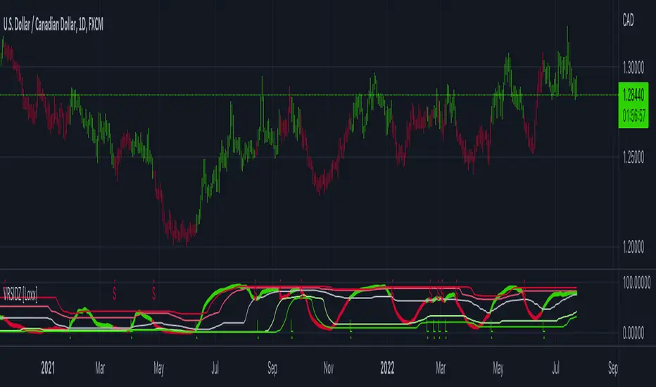
Natural Market Mirror (NMM) and NMAs w/ Dynamic Zones [Loxx]Natural Market Mirror (NMM) and NMAs w/ Dynamic Zones is a very complex indicator derived from Sloman's Ocean Theory. This indicator contains 3 core outputs and those outputs, depending on the one you select to be used to crate a long/short signal, will be highlighted and bound by Dynamic Zones. Pre-smoothing of source input is available, you only need to increase the period length to greater than 1. The smoothing algorithm used here it's Ehlers Two-pole Super Smoother. This indicator should be used as you would use the popular QQE, the difference being this indicator is multi-level momentum adaptive, and QQE is fixed RSI-based. This indicator is multilayer adaptive.
The three core indicators calculations are as follows:
NMM = Natural Market Mirror, solid line
NMF = Natural Moving Average Fast, dashed line (white when off)
NMA = Natural Moving Average Regular, dashed line (yellow when off)
Whichever one you select to be used as the signal output base, that line with increased in width and change color to match the price inputted trend. The Dynamic Zones will then readjust around that selected output and form a new bounding zone for signal output.
What is the Ocean Natural Market Mirror?
Created by Jim Sloman, the NMA is a momentum indicator that automatically adjusts to volatility without being programed to do so. For more info, read his guide "Ocean Theory, an Introduction"
What is the Ocean Natural Moving Average?
Also created by Jim Sloman, the NMA is a moving average that automatically adjusts to volatility.
What are Dynamic Zones?
As explained in "Stocks & Commodities V15:7 (306-310): Dynamic Zones by Leo Zamansky, Ph .D., and David Stendahl"
Most indicators use a fixed zone for buy and sell signals. Here’ s a concept based on zones that are responsive to past levels of the indicator.
One approach to active investing employs the use of oscillators to exploit tradable market trends. This investing style follows a very simple form of logic: Enter the market only when an oscillator has moved far above or below traditional trading lev- els. However, these oscillator- driven systems lack the ability to evolve with the market because they use fixed buy and sell zones. Traders typically use one set of buy and sell zones for a bull market and substantially different zones for a bear market. And therein lies the problem.
Once traders begin introducing their market opinions into trading equations, by changing the zones, they negate the system’s mechanical nature. The objective is to have a system automatically define its own buy and sell zones and thereby profitably trade in any market — bull or bear. Dynamic zones offer a solution to the problem of fixed buy and sell zones for any oscillator-driven system.
An indicator’s extreme levels can be quantified using statistical methods. These extreme levels are calculated for a certain period and serve as the buy and sell zones for a trading system. The repetition of this statistical process for every value of the indicator creates values that become the dynamic zones. The zones are calculated in such a way that the probability of the indicator value rising above, or falling below, the dynamic zones is equal to a given probability input set by the trader.
To better understand dynamic zones, let's first describe them mathematically and then explain their use. The dynamic zones definition:
Find V such that:
For dynamic zone buy: P{X <= V}=P1
For dynamic zone sell: P{X >= V}=P2
where P1 and P2 are the probabilities set by the trader, X is the value of the indicator for the selected period and V represents the value of the dynamic zone.
The probability input P1 and P2 can be adjusted by the trader to encompass as much or as little data as the trader would like. The smaller the probability, the fewer data values above and below the dynamic zones. This translates into a wider range between the buy and sell zones. If a 10% probability is used for P1 and P2, only those data values that make up the top 10% and bottom 10% for an indicator are used in the construction of the zones. Of the values, 80% will fall between the two extreme levels. Because dynamic zone levels are penetrated so infrequently, when this happens, traders know that the market has truly moved into overbought or oversold territory.
Calculating the Dynamic Zones
The algorithm for the dynamic zones is a series of steps. First, decide the value of the lookback period t. Next, decide the value of the probability Pbuy for buy zone and value of the probability Psell for the sell zone.
For i=1, to the last lookback period, build the distribution f(x) of the price during the lookback period i. Then find the value Vi1 such that the probability of the price less than or equal to Vi1 during the lookback period i is equal to Pbuy. Find the value Vi2 such that the probability of the price greater or equal to Vi2 during the lookback period i is equal to Psell. The sequence of Vi1 for all periods gives the buy zone. The sequence of Vi2 for all periods gives the sell zone.
In the algorithm description, we have: Build the distribution f(x) of the price during the lookback period i. The distribution here is empirical namely, how many times a given value of x appeared during the lookback period. The problem is to find such x that the probability of a price being greater or equal to x will be equal to a probability selected by the user. Probability is the area under the distribution curve. The task is to find such value of x that the area under the distribution curve to the right of x will be equal to the probability selected by the user. That x is the dynamic zone.
Included
Bar coloring
3 types of signal output options
Alerts
Loxx's Expanded Source Types
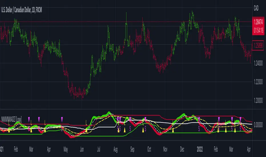
Dynamic Zone of Bollinger Band Stops Line [Loxx]Dynamic Zone of Bollinger Band Stops Line is a Bollinger Band indicator with Dynamic Zones. This indicator serves as both a trend indicator and a dynamic stop-loss indicator.
What are Bollinger Bands?
A Bollinger Band is a technical analysis tool defined by a set of trendlines plotted two standard deviations (positively and negatively) away from a simple moving average (SMA) of a security's price, but which can be adjusted to user preferences.
Bollinger Bands were developed and copyrighted by famous technical trader John Bollinger, designed to discover opportunities that give investors a higher probability of properly identifying when an asset is oversold or overbought.
What are Dynamic Zones?
As explained in "Stocks & Commodities V15:7 (306-310): Dynamic Zones by Leo Zamansky, Ph .D., and David Stendahl"
Most indicators use a fixed zone for buy and sell signals. Here’ s a concept based on zones that are responsive to past levels of the indicator.
One approach to active investing employs the use of oscillators to exploit tradable market trends. This investing style follows a very simple form of logic: Enter the market only when an oscillator has moved far above or below traditional trading lev- els. However, these oscillator- driven systems lack the ability to evolve with the market because they use fixed buy and sell zones. Traders typically use one set of buy and sell zones for a bull market and substantially different zones for a bear market. And therein lies the problem.
Once traders begin introducing their market opinions into trading equations, by changing the zones, they negate the system’s mechanical nature. The objective is to have a system automatically define its own buy and sell zones and thereby profitably trade in any market — bull or bear. Dynamic zones offer a solution to the problem of fixed buy and sell zones for any oscillator-driven system.
An indicator’s extreme levels can be quantified using statistical methods. These extreme levels are calculated for a certain period and serve as the buy and sell zones for a trading system. The repetition of this statistical process for every value of the indicator creates values that become the dynamic zones. The zones are calculated in such a way that the probability of the indicator value rising above, or falling below, the dynamic zones is equal to a given probability input set by the trader.
To better understand dynamic zones, let's first describe them mathematically and then explain their use. The dynamic zones definition:
Find V such that:
For dynamic zone buy: P{X <= V}=P1
For dynamic zone sell: P{X >= V}=P2
where P1 and P2 are the probabilities set by the trader, X is the value of the indicator for the selected period and V represents the value of the dynamic zone.
The probability input P1 and P2 can be adjusted by the trader to encompass as much or as little data as the trader would like. The smaller the probability, the fewer data values above and below the dynamic zones. This translates into a wider range between the buy and sell zones. If a 10% probability is used for P1 and P2, only those data values that make up the top 10% and bottom 10% for an indicator are used in the construction of the zones. Of the values, 80% will fall between the two extreme levels. Because dynamic zone levels are penetrated so infrequently, when this happens, traders know that the market has truly moved into overbought or oversold territory.
Calculating the Dynamic Zones
The algorithm for the dynamic zones is a series of steps. First, decide the value of the lookback period t. Next, decide the value of the probability Pbuy for buy zone and value of the probability Psell for the sell zone.
For i=1, to the last lookback period, build the distribution f(x) of the price during the lookback period i. Then find the value Vi1 such that the probability of the price less than or equal to Vi1 during the lookback period i is equal to Pbuy. Find the value Vi2 such that the probability of the price greater or equal to Vi2 during the lookback period i is equal to Psell. The sequence of Vi1 for all periods gives the buy zone. The sequence of Vi2 for all periods gives the sell zone.
In the algorithm description, we have: Build the distribution f(x) of the price during the lookback period i. The distribution here is empirical namely, how many times a given value of x appeared during the lookback period. The problem is to find such x that the probability of a price being greater or equal to x will be equal to a probability selected by the user. Probability is the area under the distribution curve. The task is to find such value of x that the area under the distribution curve to the right of x will be equal to the probability selected by the user. That x is the dynamic zone.
Included
Bar coloring
Signals
Alerts
3 types of signal smoothing