ابحث في النصوص البرمجية عن "法国市值最大的10家公司"


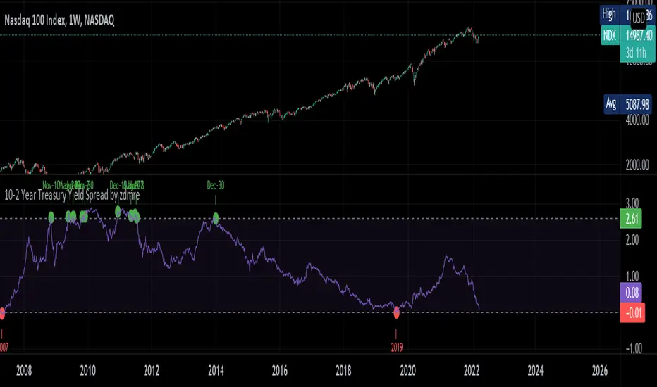
10-2 Year Treasury Yield Spread by zdmreLong-term bond yield reflects inflation. Short-term bond yields are tools used to predict Fed's interest rate policy. Spread between the two represents four cycles of an economy.
1. Growth
Short-term yield rises as interest rates rise. Spread narrows.
2. Slow growth
Central bank raises interest rates faster and short-term yield exceeds long-term yield. Spread turns negative.
3. Recession
High interest rates lead to more defaults. Inflation caps consumption. Central bank lowers interest rate to stimulate the economy and short-term yield falls. Spread widens.
4. Recovery
Central bank continues easing. Spread remains wide and yield curve remains steep.
0 = Recession Risk
2.6 = Recovery Plan
DYOR
6 Figures Scalping 2x MACD10-11-2019
This script plots a double MACD in a new indicator pane
The default settings:
Pink = STD MACD , settings 12-26-9
Green - Fast MACD, settings 5-15-1
The MACD settings can be changed in the indicators setting window

10/20/50/100/200 SMA'sMultiple MA's to get a good feel for momentum and interim supports and resistances


Moving Average x10 (SMA, EMA)10 configurable Simple and Exponential moving averages combined in one indicator
SMA RIBBON10 SMA's arranged in a ribbon. Color coded depending on price close. Free to use, open source. As seen in some charts.

10Y Bond Yield Spread (beta)10-Year Bond Yield Spread using Quandl data
See also:
- seekingalpha.com
- www.babypips.com
- www.forexfactory.com

10 Simple & 6 Exponential Moving Averages (w/ 18 day,week,month)* This is for the trader who wants tons of moving averages on their chart from one indicator
* Using the options, you should be able ot turn off some of them if the screen is too noisy for you
* You should also be able to change colors and thickness of the bars
* The thicker bars are for longer term averages
* This version is similar to my other script except it adds the 18 day, 18 week, and 18 Month SMa
* I added them after watching ira Epstein's YouTube videos
* Let me know if there are any bugs or things that need to be change

Support and Resistance levels from Options DataINTRODUCTION
This script is designed to visualize key support and resistance levels derived from options data on TradingView charts. It overlays lines, labels, and boxes to highlight levels such as Put Walls (gamma support), Call Walls (gamma resistance), Gamma Flip points, Vanna levels, and more.
These levels are intended to help traders identify potential areas of price magnetism, reversal, or breakout based on options market dynamics. All calculations and visualizations are based on user-provided data pasted into the input field, as Pine Script cannot directly fetch external options data due to platform limitations (explained below).
For convenience, my website allows users to interact with a bot that will generate the string for up to 30 tickers at once getting nearly real-time data on demand (data is cached for 15min). With the output string pasted into this indicator, it's a bliss to shuffle through your portfolio and see those levels for each ticker.
The script is open-source under TradingView's terms, allowing users to study, modify, and improve it. It draws inspiration from common options-derived metrics like gamma exposure and vanna, which are widely discussed in financial literature. No external code is copied without rights; all logic is original or based on standard mathematical formulas.
How the Options Levels Are Calculated
The levels displayed by this script are not computed within Pine Script itself—instead, they rely on pre-calculated values provided by the user (via a pasted data string). These values are derived from options chain data fetched from financial APIs (e.g., using libraries like yfinance in Python). Here's a step-by-step overview of how these levels are generally calculated externally before being input into the script:
Fetching Options Data:
Historical and current options chain data for a ticker (e.g., strikes, open interest, volume, implied volatility, expirations) is retrieved for near-term expirations (e.g., up to 90 days).
Current stock price is obtained from recent history.
Gamma Support (Put Wall) and Resistance (Call Wall):
Gamma Calculation: For each option, gamma (the rate of change of delta) is computed using the Black-Scholes formula:
gamma = N'(d1) / (S * sigma * sqrt(T))
where S is the stock price, K is the strike, T is time to expiration (in years), sigma is implied volatility, r is the risk-free rate (e.g., 0.0445), and N'(d1) is the normal probability density function.
Weighted gamma is multiplied by open interest and aggregated by strike.
The Put Wall is the strike below the current price with the highest weighted gamma from puts (acting as support).
The Call Wall is the strike above the current price with the highest weighted gamma from calls (acting as resistance).
Short-term versions focus on strikes closer to the money (e.g., within 10-15% of the price).
Gamma Flip Level:
Net dealer gamma exposure (GEX) is calculated across all strikes:
GEX = sum (gamma * OI * 100 * S^2 * sign * decay)
where sign is +1 for calls/-1 for puts, and decay is 1 / sqrt(T).
The flip point is the price where net GEX changes sign (from positive to negative or vice versa), interpolated between strikes.
Vanna Levels:
Vanna (sensitivity of delta to volatility) is calculated:
vanna = -N'(d1) * d2 / sigma
where d2 = d1 - sigma * sqrt(T).
Weighted by open interest, the highest positive and negative vanna strikes are identified.
Other Levels:
S1/R1: Significant strikes with high combined open interest and volume (80% OI + 20% volume), below/above price for support/resistance.
Implied Move: ATM implied volatility scaled by S * sigma * sqrt(d/365) (e.g., for 7 days).
Call/Put Ratio: Total call contracts divided by put contracts (OI + volume).
IV Percentage: Average ATM implied volatility.
Options Activity Level: Average contracts per unique strike, binned into levels (0-4).
Stop Loss: Dynamically set below the lowest support (e.g., Put Wall, Gamma Flip), adjusted by IV (tighter in low IV).
Fib Target: 1.618 extension from Put Wall to Call Wall range.
Previous day levels are stored for comparison (e.g., to detect Call Wall movement >2.5% for alerts).
Effect as Support and Resistance in Technical Trading
Options levels like gamma walls influence price action due to market maker hedging:
Put Wall (Gamma Support): High put gamma below price creates a "magnet" effect—market makers buy stock as price falls, providing support. Traders might look for bounces here as entry points for longs.
Call Wall (Gamma Resistance): High call gamma above price leads to selling pressure from hedging, acting as resistance. Rejections here could signal trims, sells or even shorts.
Gamma Flip: Where gamma exposure flips sign, often a volatility pivot—crossing it can accelerate moves (bullish above, bearish below).
Vanna Levels: Positive/negative vanna indicate volatility sensitivity; crosses may signal regime shifts.
Implied Move: Shows expected range; prices outside suggest overextension.
S1/R1 and Fib Target: Volume/OI clusters act as classic S/R; Fib extensions project upside targets post-breakout.
In trading, these are not guarantees—combine with TA (e.g., volume, trends). High activity levels imply stronger effects; low CP ratio suggests bearish sentiment. Alerts trigger on proximities/crosses for awareness, not advice.
Limitations of the TradingView Platform for Data Pulling
TradingView's Pine Script is sandboxed for security and performance:
No direct internet access or API calls (e.g., can't fetch yfinance data in-script).
Limited to chart data/symbol info; no real-time options chains.
Inputs are static per load; updates require manual pasting.
Caching isn't persistent across sessions.
This prevents dynamic data pulling, ensuring scripts remain lightweight but requiring external tools for fresh data.
Creative Solution for On-Demand Data Pulling
To overcome these limitations, users can use external tools or scripts (e.g., Python-based) to fetch and compute levels on demand. The tool processes tickers, generates a formatted string (e.g., "TICKER:level1,level2,...;TIMESTAMP:unix;"), and users paste it into the script's input. This keeps data fresh without violating platform rules, as computation happens off-platform. For example, run a local script to query APIs and output the string—adaptable for any ticker.
Script Functionality Breakdown
Inputs: Custom data string (parsed for levels/timestamp); toggles for short-term/previous/Vanna/stop loss; style options (colors, transparency).
Parsing: Extracts levels for the chart symbol; gets timestamp for "updated ago" display.
Drawing: Lines/labels for levels; boxes for gamma zones/implied move; clears old elements on updates.
Info Panel: Top-right summary with metrics (CP ratio, IV, distances, activity); emojis for quick status.
Alerts: Conditions for proximities, crosses, bounces (e.g., 0.5% bounce from Put Wall).
Performance: Uses vars for persistence; efficient for real-time.
This script is educational—test thoroughly. Not financial advice; past performance isn't indicative of future results. Feedback welcome via TradingView comments.

Quad Stochastic Div (Latching Quad)This script combines 4 stochastic lines, plotting only the %D lines.
(9,3)(14,3)(40,4)(60,10)
When all 4 are oversold or overbought, a buy or sell background is painted. When the slowest moving stochastic finally rotates back towards the center, the background will unlatch. This script also marks most divergences made between the chart and the 2 faster moving stochastic lines. White markers for the 9,3 and orange markers for the 14,4. Tradable signals are both orange and white divergence occurring on the same pivot, or either divergence leading out of a rotation. Generally more useful for scalping 1-5m charts.
I also built out some strength ratings to attempt to classify the divergences against one another, but this didn't seem to have much value in practice so by default the tags are turned off.
This indicator is helpful for anyone interested in daytradingrockstar on youtube's quad stochastic strategy.

Ultimate Pattern ScannerSmart Pattern Scanner Pro - Complete Study Guide
The Smart Pattern Scanner Pro is an advanced candlestick pattern recognition indicator that automatically detects over 30 traditional Japanese candlestick patterns across multiple timeframes simultaneously. It combines pattern recognition with volume analysis and trend confirmation to provide traders with comprehensive reversal and continuation signals.
Core Features:
• 30+ Candlestick Patterns: Complete library of traditional patterns
• Multi-Timeframe Scanning: Simultaneous analysis across up to 7 timeframes
• Volume Integration: Buy/sell volume analysis with pattern confirmation
• Trend Filtering: SMA-based trend confirmation for pattern validity
• Real-Time Dashboard: Professional interface with customizable display
• Alert System: Automated notifications when patterns are detected
________________________________________
Candlestick Pattern Categories
Reversal Patterns (Bullish)
Single Candle Patterns
1. Hammer
o Formation: Small body at top, long lower shadow (2x body size)
o Signal: Bullish reversal after downtrend
o Reliability: High when confirmed with volume
o Entry: Above hammer high with stop below low
2. Inverted Hammer
o Formation: Small body at bottom, long upper shadow
o Signal: Potential bullish reversal (needs confirmation)
o Reliability: Medium (requires next candle confirmation)
o Entry: Confirmed breakout above pattern
3. Dragonfly Doji
o Formation: Open = Close, long lower shadow, no upper shadow
o Signal: Strong bullish reversal signal
o Reliability: High in downtrends
o Entry: Above doji high with tight stop
4. Long Lower Shadow
o Formation: Lower shadow 2x body length
o Signal: Rejection of lower prices, bullish sentiment
o Reliability: Medium to high with volume
o Entry: Above candle high
Multi-Candle Patterns
1. Bullish Engulfing
o Formation: Large white candle completely engulfs previous black candle
o Signal: Strong bullish reversal
o Reliability: Very high with volume confirmation
o Entry: Above engulfing candle high
2. Morning Star
o Formation: 3-candle pattern (down, small, up)
o Signal: Major bullish reversal
o Reliability: Excellent (one of most reliable patterns)
o Entry: Above third candle high
3. Morning Doji Star
o Formation: Like Morning Star but middle candle is doji
o Signal: Strong bullish reversal
o Reliability: Very high
o Entry: Above third candle close
4. Piercing Pattern
o Formation: White candle opens below previous low, closes above midpoint
o Signal: Bullish reversal
o Reliability: High when closing >50% into previous candle
o Entry: Above piercing candle high
5. Bullish Harami
o Formation: Small white candle within previous large black candle
o Signal: Potential bullish reversal
o Reliability: Medium (needs confirmation)
o Entry: Above mother candle high
Reversal Patterns (Bearish)
Single Candle Patterns
1. Shooting Star
o Formation: Small body at bottom, long upper shadow
o Signal: Bearish reversal after uptrend
o Reliability: High with volume confirmation
o Entry: Below shooting star low
2. Hanging Man
o Formation: Like hammer but appears in uptrend
o Signal: Potential bearish reversal
o Reliability: Medium (needs confirmation)
o Entry: Below hanging man low
3. Gravestone Doji
o Formation: Open = Close, long upper shadow, no lower shadow
o Signal: Strong bearish reversal
o Reliability: High in uptrends
o Entry: Below doji low
4. Long Upper Shadow
o Formation: Upper shadow 2x body length
o Signal: Rejection of higher prices
o Reliability: Medium to high
o Entry: Below candle low
Multi-Candle Patterns
1. Bearish Engulfing
o Formation: Large black candle engulfs previous white candle
o Signal: Strong bearish reversal
o Reliability: Very high
o Entry: Below engulfing candle low
2. Evening Star
o Formation: 3-candle pattern (up, small, down)
o Signal: Major bearish reversal
o Reliability: Excellent
o Entry: Below third candle low
3. Dark Cloud Cover
o Formation: Black candle opens above previous high, closes below midpoint
o Signal: Bearish reversal
o Reliability: High when closing <50% into previous candle
o Entry: Below dark cloud low
Continuation Patterns
1. Rising Three Methods
o Formation: White candle, 3 small declining candles, white candle
o Signal: Bullish continuation
o Reliability: High in strong uptrends
2. Falling Three Methods
o Formation: Black candle, 3 small rising candles, black candle
o Signal: Bearish continuation
o Reliability: High in strong downtrends
Indecision Patterns
1. Doji
o Formation: Open = Close (or very close)
o Signal: Market indecision, potential reversal
o Reliability: Context-dependent
2. Spinning Tops
o Formation: Small body with upper and lower shadows
o Signal: Market indecision
o Reliability: Low without confirmation
________________________________________
Multi-Timeframe Analysis
Timeframe Hierarchy Strategy
Primary Analysis Flow:
1. Higher Timeframe (Daily/Weekly): Establish overall trend direction
2. Intermediate Timeframe (4H/1H): Identify key support/resistance levels
3. Lower Timeframe (15M/5M): Precise entry and exit timing
Configuration Guidelines:
• Scalping: 1M, 3M, 5M, 15M, 30M
• Day Trading: 5M, 15M, 30M, 1H, 4H
• Swing Trading: 1H, 4H, 1D, 1W
• Position Trading: 4H, 1D, 1W, 1M
Pattern Confluence Rules:
1. High Probability Setup: Same pattern type appears on 3+ timeframes
2. Trend Alignment: Reversal patterns should align with higher timeframe structure
3. Volume Confirmation: Strong volume on pattern timeframe and higher timeframes
________________________________________
Volume Analysis Integration
Volume Components:
1. Buy Volume: Volume when close > open (green candles)
2. Sell Volume: Volume when close ≤ open (red candles)
3. Volume Ratio: Current volume / 20-period moving average
4. Progress Indicator: Visual representation of volume strength
Volume Signal Interpretation:
• Ratio >1.5: Strong volume confirmation
• Ratio 1.0-1.5: Moderate volume support
• Ratio <1.0: Weak volume (pattern less reliable)
Volume Analysis Rules:
1. Bullish Patterns: Require strong buy volume for confirmation
2. Bearish Patterns: Require strong sell volume for confirmation
3. Volume Divergence: When pattern and volume disagree, favor volume
4. Volume Spikes: Ratios >2.0 indicate institutional interest
________________________________________
Live Market Application
Step 1: Dashboard Setup
1. Position Selection: Choose optimal table position for your layout
2. Timeframe Configuration: Set relevant timeframes for your strategy
3. Volume Analysis: Enable for confirmation signals
4. Progress Indicators: Enable for visual signal strength
Step 2: Pattern Identification Process
Real-Time Scanning:
1. Monitor Multiple Timeframes: Check all configured timeframes simultaneously
2. Pattern Priority: Focus on patterns appearing on higher timeframes first
3. Signal Confluence: Look for patterns appearing across multiple timeframes
4. Volume Confirmation: Verify adequate volume support
Pattern Validation:
1. Trend Context: Ensure pattern aligns with overall market structure
2. Support/Resistance: Check if pattern forms at key levels
3. Market Conditions: Consider overall market volatility and sentiment
4. Time of Day: Be aware of session characteristics (open, close, lunch)
Step 3: Entry Decision Matrix
High Probability Entries:
• Pattern on 3+ timeframes
• Strong volume confirmation (ratio >1.5)
• Trend alignment with higher timeframes
• Formation at key support/resistance
Medium Probability Entries:
• Pattern on 2 timeframes
• Moderate volume (ratio 1.0-1.5)
• Partial trend alignment
• Formation in trending market
Low Probability Entries:
• Single timeframe pattern
• Weak volume (ratio <1.0)
• Counter-trend formation
• Choppy/sideways market
________________________________________
Pattern Reliability Assessment
Tier 1 Patterns (Highest Reliability - 70-80% success rate):
• Morning Star / Evening Star
• Bullish/Bearish Engulfing
• Three White Soldiers / Three Black Crows
• Hammer (in strong downtrend)
• Shooting Star (in strong uptrend)
Tier 2 Patterns (High Reliability - 60-70% success rate):
• Piercing Pattern / Dark Cloud Cover
• Morning/Evening Doji Star
• Harami patterns
• Abandoned Baby
• Kicking patterns
Tier 3 Patterns (Moderate Reliability - 50-60% success rate):
• Doji patterns
• Tweezer Tops/Bottoms
• Window patterns
• Tasuki Gap patterns
• Marubozu patterns
Tier 4 Patterns (Lower Reliability - 40-50% success rate):
• Spinning Tops
• Long shadow patterns (single)
• Neutral doji formations
• Single candle continuation patterns
________________________________________
Trading Strategies
Strategy 1: Multi-Timeframe Reversal
Objective: Catch major trend reversals using high-reliability patterns
Rules:
1. Wait for Tier 1 patterns on Daily + 4H timeframes
2. Require volume ratio >1.5 on both timeframes
3. Enter on 1H confirmation candle
4. Stop loss below/above pattern extreme
5. Target 2:1 or 3:1 risk-reward ratio
Strategy 2: Intraday Scalping
Objective: Quick profits from short-term pattern formations
Rules:
1. Focus on 5M and 15M timeframes
2. Trade only Tier 1 and Tier 2 patterns
3. Require volume confirmation
4. Quick exits (10-30 pip targets)
5. Tight stops (5-15 pips)
Strategy 3: Swing Trading
Objective: Multi-day position holding based on pattern signals
Rules:
1. Use Daily and Weekly timeframes
2. Focus on major reversal patterns
3. Combine with fundamental analysis
4. Wider stops (2-5% of entry price)
5. Hold for 5-20 trading days
Strategy 4: Trend Continuation
Objective: Enter trending markets using continuation patterns
Rules:
1. Identify strong trends on higher timeframes
2. Wait for continuation patterns on lower timeframes
3. Enter in direction of main trend
4. Trail stops using pattern lows/highs
5. Pyramid positions on additional patterns
________________________________________
Risk Management
Position Sizing Rules:
1. Tier 1 Patterns: Risk up to 2% of account
2. Tier 2 Patterns: Risk up to 1.5% of account
3. Tier 3 Patterns: Risk up to 1% of account
4. Tier 4 Patterns: Risk up to 0.5% of account
Stop Loss Guidelines:
1. Reversal Patterns: Stop beyond pattern extreme + 1 ATR
2. Continuation Patterns: Stop at pattern invalidation level
3. Doji Patterns: Tight stops due to indecision nature
4. Multi-Candle Patterns: Use pattern range for stop placement
Take Profit Strategies:
1. Conservative: 1:1 risk-reward ratio
2. Moderate: 2:1 risk-reward ratio
3. Aggressive: 3:1 risk-reward ratio
4. Trailing: Move stops to breakeven after 1:1 achieved
________________________________________
Limitations and Considerations
Technical Limitations:
1. Pattern Subjectivity: Slight variations in pattern interpretation
2. Market Context Dependency: Patterns perform differently in various market conditions
3. False Signals: Not all patterns lead to expected price moves
4. Lagging Nature: Patterns are confirmed after formation is complete
Market Condition Considerations:
1. Trending Markets: Continuation patterns more reliable than reversals
2. Range-Bound Markets: Reversal patterns at extremes more effective
3. High Volatility: Patterns may not develop properly
4. News Events: Fundamental factors can override technical patterns
Optimal Usage Conditions:
1. Liquid Markets: Adequate volume and participation
2. Normal Volatility: Not during extreme market stress
3. Clear Market Structure: Defined support and resistance levels
4. Multiple Timeframe Alignment: Confluence across timeframes
When NOT to Trade Patterns:
1. Major News Releases: Economic announcements can invalidate patterns
2. Market Holidays: Reduced participation affects reliability
3. Extreme Volatility: VIX >30 or similar stress indicators
4. Gap Openings: Large gaps can negate pattern significance
________________________________________
Risk Disclaimer
CRITICAL WARNING FROM aiTrendview
TRADING FINANCIAL INSTRUMENTS INVOLVES SUBSTANTIAL RISK OF LOSS
This Smart Pattern Scanner Pro indicator ("the Indicator") is provided for educational and analytical purposes only. By using this indicator, you acknowledge and accept the following terms and conditions:
No Financial Advice
• NOT INVESTMENT ADVICE: This indicator does not constitute financial, investment, or trading advice
• NO RECOMMENDATIONS: Pattern signals are not recommendations to buy or sell any financial instrument
• EDUCATIONAL TOOL: Designed for learning technical analysis concepts and pattern recognition
• INDEPENDENT RESEARCH REQUIRED: Always conduct your own thorough analysis before making trading decisions
Substantial Trading Risks
• CAPITAL LOSS RISK: You may lose some or all of your trading capital
• LEVERAGE DANGERS: Margin trading can amplify losses beyond your initial investment
• MARKET VOLATILITY: Financial markets are inherently unpredictable and can move against any analysis
• PATTERN FAILURE: Candlestick patterns fail frequently and do not guarantee profitable outcomes
• FALSE SIGNALS: The indicator may generate incorrect or misleading signals
Technical Analysis Limitations
• NOT PREDICTIVE: Candlestick patterns analyze past price action, not future movements
• SUBJECTIVE INTERPRETATION: Pattern recognition can vary between traders and market conditions
• CONTEXT DEPENDENT: Patterns must be analyzed within broader market context
• NO GUARANTEE: No technical analysis method guarantees trading success
• STATISTICAL PROBABILITY: Even high-reliability patterns fail 20-30% of the time
User Responsibilities
• SOLE RESPONSIBILITY: You are entirely responsible for all trading decisions and outcomes
• RISK MANAGEMENT: Implement appropriate position sizing and stop-loss strategies
• PROFESSIONAL CONSULTATION: Seek advice from qualified financial professionals
• REGULATORY COMPLIANCE: Ensure compliance with local financial regulations
• CONTINUOUS EDUCATION: Maintain ongoing education in market analysis and risk management
Indicator Limitations
• SOFTWARE BUGS: Technical glitches or calculation errors may occur
• DATA DEPENDENCY: Relies on accurate price and volume data feeds
• PLATFORM LIMITATIONS: Subject to TradingView platform capabilities and restrictions
• VERSION UPDATES: Functionality may change with future updates
• COMPATIBILITY: May not work optimally with all chart configurations
Volume Analysis Limitations
• DATA ACCURACY: Volume data may be incomplete or delayed
• MARKET VARIATIONS: Volume patterns differ across markets and instruments
• INSTITUTIONAL ACTIVITY: Cannot guarantee detection of all institutional trading
• LIQUIDITY FACTORS: Low liquidity markets may produce unreliable volume signals
Multi-Timeframe Considerations
• CONFLICTING SIGNALS: Different timeframes may show contradictory patterns
• TIME SYNCHRONIZATION: Pattern timing may vary across timeframes
• COMPUTATIONAL LOAD: Multiple timeframe analysis may affect performance
• COMPLEXITY RISK: More data does not necessarily mean better decisions
Specific Trading Warnings
Pattern-Specific Risks:
1. Doji Patterns: Indicate indecision, not directional conviction
2. Single Candle Patterns: Generally less reliable than multi-candle formations
3. Continuation Patterns: May signal trend exhaustion rather than continuation
4. Gap Patterns: Subject to overnight and weekend gap risks
Market Condition Risks:
1. News Events: Fundamental factors can invalidate any technical pattern
2. Market Manipulation: Large players can create false pattern signals
3. Algorithmic Trading: High-frequency trading can distort traditional patterns
4. Market Crashes: Extreme events render technical analysis ineffective
Psychological Trading Risks:
1. Overconfidence: Successful patterns may lead to excessive risk-taking
2. Pattern Addiction: Over-reliance on patterns without broader analysis
3. Confirmation Bias: Seeing patterns that don't actually exist
4. Emotional Trading: Fear and greed can override pattern discipline
Legal and Regulatory Disclaimers
Intellectual Property:
• COPYRIGHT PROTECTION: This indicator is protected by copyright law
• AUTHORIZED USE ONLY: Use only as permitted by TradingView terms of service
• NO REDISTRIBUTION: Unauthorized copying or redistribution is prohibited
• MODIFICATION RESTRICTIONS: Code modifications may void any support or warranties
Regulatory Compliance:
• LOCAL LAWS: Ensure compliance with your jurisdiction's financial regulations
• LICENSING REQUIREMENTS: Some jurisdictions require licenses for trading or advisory activities
• TAX OBLIGATIONS: Trading profits/losses may have tax implications
• REPORTING REQUIREMENTS: Some jurisdictions require reporting of trading activities
Limitation of Liability:
• NO LIABILITY: aiTrendview accepts no liability for any losses, damages, or adverse outcomes
• INDIRECT DAMAGES: Not liable for consequential, incidental, or punitive damages
• MAXIMUM LIABILITY: Limited to amount paid for indicator access (if any)
• FORCE MAJEURE: Not responsible for events beyond reasonable control
Final Warnings and Recommendations
Before Using This Indicator:
1. DEMO TRADING: Practice extensively with paper trading before risking real money
2. EDUCATION: Thoroughly understand candlestick pattern theory and market dynamics
3. RISK ASSESSMENT: Honestly assess your risk tolerance and financial situation
4. PROFESSIONAL ADVICE: Consult with qualified financial advisors
5. START SMALL: Begin with minimal position sizes to test strategies
Red Flags - Do NOT Trade If:
• You cannot afford to lose the money you're risking
• You're experiencing financial stress or pressure
• You're trading emotionally or impulsively
• You don't understand the patterns or market mechanics
• You're using borrowed money or credit to trade
• You're treating trading as gambling rather than calculated risk-taking
Emergency Procedures:
• STOP TRADING immediately if experiencing significant losses
• SEEK HELP if trading is affecting your mental health or relationships
• REVIEW STRATEGY after any series of losses
• TAKE BREAKS from trading to maintain perspective
• PROFESSIONAL HELP: Contact financial counselors if needed
Acknowledgment Required
By using the Smart Pattern Scanner Pro indicator, you explicitly acknowledge that:
1. You have read and understood this entire disclaimer
2. You accept full responsibility for all trading decisions and outcomes
3. You understand the substantial risks involved in financial trading
4. You will not hold aiTrendview liable for any losses or damages
5. You will use this tool only for educational and personal analysis purposes
6. You will comply with all applicable laws and regulations
7. You will implement appropriate risk management practices
8. You understand that past performance does not predict future results
REMEMBER: The most important rule in trading is capital preservation. No pattern, indicator, or strategy is worth risking your financial well-being.
________________________________________
Disclaimer from aiTrendview.com
The content provided in this blog post is for educational and training purposes only. It is not intended to be, and should not be construed as, financial, investment, or trading advice. All charting and technical analysis examples are for illustrative purposes. Trading and investing in financial markets involve substantial risk of loss and are not suitable for every individual. Before making any financial decisions, you should consult with a qualified financial professional to assess your personal financial situation.

Markov Chain [3D] | FractalystWhat exactly is a Markov Chain?
This indicator uses a Markov Chain model to analyze, quantify, and visualize the transitions between market regimes (Bull, Bear, Neutral) on your chart. It dynamically detects these regimes in real-time, calculates transition probabilities, and displays them as animated 3D spheres and arrows, giving traders intuitive insight into current and future market conditions.
How does a Markov Chain work, and how should I read this spheres-and-arrows diagram?
Think of three weather modes: Sunny, Rainy, Cloudy.
Each sphere is one mode. The loop on a sphere means “stay the same next step” (e.g., Sunny again tomorrow).
The arrows leaving a sphere show where things usually go next if they change (e.g., Sunny moving to Cloudy).
Some paths matter more than others. A more prominent loop means the current mode tends to persist. A more prominent outgoing arrow means a change to that destination is the usual next step.
Direction isn’t symmetric: moving Sunny→Cloudy can behave differently than Cloudy→Sunny.
Now relabel the spheres to markets: Bull, Bear, Neutral.
Spheres: market regimes (uptrend, downtrend, range).
Self‑loop: tendency for the current regime to continue on the next bar.
Arrows: the most common next regime if a switch happens.
How to read: Start at the sphere that matches current bar state. If the loop stands out, expect continuation. If one outgoing path stands out, that switch is the typical next step. Opposite directions can differ (Bear→Neutral doesn’t have to match Neutral→Bear).
What states and transitions are shown?
The three market states visualized are:
Bullish (Bull): Upward or strong-market regime.
Bearish (Bear): Downward or weak-market regime.
Neutral: Sideways or range-bound regime.
Bidirectional animated arrows and probability labels show how likely the market is to move from one regime to another (e.g., Bull → Bear or Neutral → Bull).
How does the regime detection system work?
You can use either built-in price returns (based on adaptive Z-score normalization) or supply three custom indicators (such as volume, oscillators, etc.).
Values are statistically normalized (Z-scored) over a configurable lookback period.
The normalized outputs are classified into Bull, Bear, or Neutral zones.
If using three indicators, their regime signals are averaged and smoothed for robustness.
How are transition probabilities calculated?
On every confirmed bar, the algorithm tracks the sequence of detected market states, then builds a rolling window of transitions.
The code maintains a transition count matrix for all regime pairs (e.g., Bull → Bear).
Transition probabilities are extracted for each possible state change using Laplace smoothing for numerical stability, and frequently updated in real-time.
What is unique about the visualization?
3D animated spheres represent each regime and change visually when active.
Animated, bidirectional arrows reveal transition probabilities and allow you to see both dominant and less likely regime flows.
Particles (moving dots) animate along the arrows, enhancing the perception of regime flow direction and speed.
All elements dynamically update with each new price bar, providing a live market map in an intuitive, engaging format.
Can I use custom indicators for regime classification?
Yes! Enable the "Custom Indicators" switch and select any three chart series as inputs. These will be normalized and combined (each with equal weight), broadening the regime classification beyond just price-based movement.
What does the “Lookback Period” control?
Lookback Period (default: 100) sets how much historical data builds the probability matrix. Shorter periods adapt faster to regime changes but may be noisier. Longer periods are more stable but slower to adapt.
How is this different from a Hidden Markov Model (HMM)?
It sets the window for both regime detection and probability calculations. Lower values make the system more reactive, but potentially noisier. Higher values smooth estimates and make the system more robust.
How is this Markov Chain different from a Hidden Markov Model (HMM)?
Markov Chain (as here): All market regimes (Bull, Bear, Neutral) are directly observable on the chart. The transition matrix is built from actual detected regimes, keeping the model simple and interpretable.
Hidden Markov Model: The actual regimes are unobservable ("hidden") and must be inferred from market output or indicator "emissions" using statistical learning algorithms. HMMs are more complex, can capture more subtle structure, but are harder to visualize and require additional machine learning steps for training.
A standard Markov Chain models transitions between observable states using a simple transition matrix, while a Hidden Markov Model assumes the true states are hidden (latent) and must be inferred from observable “emissions” like price or volume data. In practical terms, a Markov Chain is transparent and easier to implement and interpret; an HMM is more expressive but requires statistical inference to estimate hidden states from data.
Markov Chain: states are observable; you directly count or estimate transition probabilities between visible states. This makes it simpler, faster, and easier to validate and tune.
HMM: states are hidden; you only observe emissions generated by those latent states. Learning involves machine learning/statistical algorithms (commonly Baum–Welch/EM for training and Viterbi for decoding) to infer both the transition dynamics and the most likely hidden state sequence from data.
How does the indicator avoid “repainting” or look-ahead bias?
All regime changes and matrix updates happen only on confirmed (closed) bars, so no future data is leaked, ensuring reliable real-time operation.
Are there practical tuning tips?
Tune the Lookback Period for your asset/timeframe: shorter for fast markets, longer for stability.
Use custom indicators if your asset has unique regime drivers.
Watch for rapid changes in transition probabilities as early warning of a possible regime shift.
Who is this indicator for?
Quants and quantitative researchers exploring probabilistic market modeling, especially those interested in regime-switching dynamics and Markov models.
Programmers and system developers who need a probabilistic regime filter for systematic and algorithmic backtesting:
The Markov Chain indicator is ideally suited for programmatic integration via its bias output (1 = Bull, 0 = Neutral, -1 = Bear).
Although the visualization is engaging, the core output is designed for automated, rules-based workflows—not for discretionary/manual trading decisions.
Developers can connect the indicator’s output directly to their Pine Script logic (using input.source()), allowing rapid and robust backtesting of regime-based strategies.
It acts as a plug-and-play regime filter: simply plug the bias output into your entry/exit logic, and you have a scientifically robust, probabilistically-derived signal for filtering, timing, position sizing, or risk regimes.
The MC's output is intentionally "trinary" (1/0/-1), focusing on clear regime states for unambiguous decision-making in code. If you require nuanced, multi-probability or soft-label state vectors, consider expanding the indicator or stacking it with a probability-weighted logic layer in your scripting.
Because it avoids subjectivity, this approach is optimal for systematic quants, algo developers building backtested, repeatable strategies based on probabilistic regime analysis.
What's the mathematical foundation behind this?
The mathematical foundation behind this Markov Chain indicator—and probabilistic regime detection in finance—draws from two principal models: the (standard) Markov Chain and the Hidden Markov Model (HMM).
How to use this indicator programmatically?
The Markov Chain indicator automatically exports a bias value (+1 for Bullish, -1 for Bearish, 0 for Neutral) as a plot visible in the Data Window. This allows you to integrate its regime signal into your own scripts and strategies for backtesting, automation, or live trading.
Step-by-Step Integration with Pine Script (input.source)
Add the Markov Chain indicator to your chart.
This must be done first, since your custom script will "pull" the bias signal from the indicator's plot.
In your strategy, create an input using input.source()
Example:
//@version=5
strategy("MC Bias Strategy Example")
mcBias = input.source(close, "MC Bias Source")
After saving, go to your script’s settings. For the “MC Bias Source” input, select the plot/output of the Markov Chain indicator (typically its bias plot).
Use the bias in your trading logic
Example (long only on Bull, flat otherwise):
if mcBias == 1
strategy.entry("Long", strategy.long)
else
strategy.close("Long")
For more advanced workflows, combine mcBias with additional filters or trailing stops.
How does this work behind-the-scenes?
TradingView’s input.source() lets you use any plot from another indicator as a real-time, “live” data feed in your own script (source).
The selected bias signal is available to your Pine code as a variable, enabling logical decisions based on regime (trend-following, mean-reversion, etc.).
This enables powerful strategy modularity : decouple regime detection from entry/exit logic, allowing fast experimentation without rewriting core signal code.
Integrating 45+ Indicators with Your Markov Chain — How & Why
The Enhanced Custom Indicators Export script exports a massive suite of over 45 technical indicators—ranging from classic momentum (RSI, MACD, Stochastic, etc.) to trend, volume, volatility, and oscillator tools—all pre-calculated, centered/scaled, and available as plots.
// Enhanced Custom Indicators Export - 45 Technical Indicators
// Comprehensive technical analysis suite for advanced market regime detection
//@version=6
indicator('Enhanced Custom Indicators Export | Fractalyst', shorttitle='Enhanced CI Export', overlay=false, scale=scale.right, max_labels_count=500, max_lines_count=500)
// |----- Input Parameters -----| //
momentum_group = "Momentum Indicators"
trend_group = "Trend Indicators"
volume_group = "Volume Indicators"
volatility_group = "Volatility Indicators"
oscillator_group = "Oscillator Indicators"
display_group = "Display Settings"
// Common lengths
length_14 = input.int(14, "Standard Length (14)", minval=1, maxval=100, group=momentum_group)
length_20 = input.int(20, "Medium Length (20)", minval=1, maxval=200, group=trend_group)
length_50 = input.int(50, "Long Length (50)", minval=1, maxval=200, group=trend_group)
// Display options
show_table = input.bool(true, "Show Values Table", group=display_group)
table_size = input.string("Small", "Table Size", options= , group=display_group)
// |----- MOMENTUM INDICATORS (15 indicators) -----| //
// 1. RSI (Relative Strength Index)
rsi_14 = ta.rsi(close, length_14)
rsi_centered = rsi_14 - 50
// 2. Stochastic Oscillator
stoch_k = ta.stoch(close, high, low, length_14)
stoch_d = ta.sma(stoch_k, 3)
stoch_centered = stoch_k - 50
// 3. Williams %R
williams_r = ta.stoch(close, high, low, length_14) - 100
// 4. MACD (Moving Average Convergence Divergence)
= ta.macd(close, 12, 26, 9)
// 5. Momentum (Rate of Change)
momentum = ta.mom(close, length_14)
momentum_pct = (momentum / close ) * 100
// 6. Rate of Change (ROC)
roc = ta.roc(close, length_14)
// 7. Commodity Channel Index (CCI)
cci = ta.cci(close, length_20)
// 8. Money Flow Index (MFI)
mfi = ta.mfi(close, length_14)
mfi_centered = mfi - 50
// 9. Awesome Oscillator (AO)
ao = ta.sma(hl2, 5) - ta.sma(hl2, 34)
// 10. Accelerator Oscillator (AC)
ac = ao - ta.sma(ao, 5)
// 11. Chande Momentum Oscillator (CMO)
cmo = ta.cmo(close, length_14)
// 12. Detrended Price Oscillator (DPO)
dpo = close - ta.sma(close, length_20)
// 13. Price Oscillator (PPO)
ppo = ta.sma(close, 12) - ta.sma(close, 26)
ppo_pct = (ppo / ta.sma(close, 26)) * 100
// 14. TRIX
trix_ema1 = ta.ema(close, length_14)
trix_ema2 = ta.ema(trix_ema1, length_14)
trix_ema3 = ta.ema(trix_ema2, length_14)
trix = ta.roc(trix_ema3, 1) * 10000
// 15. Klinger Oscillator
klinger = ta.ema(volume * (high + low + close) / 3, 34) - ta.ema(volume * (high + low + close) / 3, 55)
// 16. Fisher Transform
fisher_hl2 = 0.5 * (hl2 - ta.lowest(hl2, 10)) / (ta.highest(hl2, 10) - ta.lowest(hl2, 10)) - 0.25
fisher = 0.5 * math.log((1 + fisher_hl2) / (1 - fisher_hl2))
// 17. Stochastic RSI
stoch_rsi = ta.stoch(rsi_14, rsi_14, rsi_14, length_14)
stoch_rsi_centered = stoch_rsi - 50
// 18. Relative Vigor Index (RVI)
rvi_num = ta.swma(close - open)
rvi_den = ta.swma(high - low)
rvi = rvi_den != 0 ? rvi_num / rvi_den : 0
// 19. Balance of Power (BOP)
bop = (close - open) / (high - low)
// |----- TREND INDICATORS (10 indicators) -----| //
// 20. Simple Moving Average Momentum
sma_20 = ta.sma(close, length_20)
sma_momentum = ((close - sma_20) / sma_20) * 100
// 21. Exponential Moving Average Momentum
ema_20 = ta.ema(close, length_20)
ema_momentum = ((close - ema_20) / ema_20) * 100
// 22. Parabolic SAR
sar = ta.sar(0.02, 0.02, 0.2)
sar_trend = close > sar ? 1 : -1
// 23. Linear Regression Slope
lr_slope = ta.linreg(close, length_20, 0) - ta.linreg(close, length_20, 1)
// 24. Moving Average Convergence (MAC)
mac = ta.sma(close, 10) - ta.sma(close, 30)
// 25. Trend Intensity Index (TII)
tii_sum = 0.0
for i = 1 to length_20
tii_sum += close > close ? 1 : 0
tii = (tii_sum / length_20) * 100
// 26. Ichimoku Cloud Components
ichimoku_tenkan = (ta.highest(high, 9) + ta.lowest(low, 9)) / 2
ichimoku_kijun = (ta.highest(high, 26) + ta.lowest(low, 26)) / 2
ichimoku_signal = ichimoku_tenkan > ichimoku_kijun ? 1 : -1
// 27. MESA Adaptive Moving Average (MAMA)
mama_alpha = 2.0 / (length_20 + 1)
mama = ta.ema(close, length_20)
mama_momentum = ((close - mama) / mama) * 100
// 28. Zero Lag Exponential Moving Average (ZLEMA)
zlema_lag = math.round((length_20 - 1) / 2)
zlema_data = close + (close - close )
zlema = ta.ema(zlema_data, length_20)
zlema_momentum = ((close - zlema) / zlema) * 100
// |----- VOLUME INDICATORS (6 indicators) -----| //
// 29. On-Balance Volume (OBV)
obv = ta.obv
// 30. Volume Rate of Change (VROC)
vroc = ta.roc(volume, length_14)
// 31. Price Volume Trend (PVT)
pvt = ta.pvt
// 32. Negative Volume Index (NVI)
nvi = 0.0
nvi := volume < volume ? nvi + ((close - close ) / close ) * nvi : nvi
// 33. Positive Volume Index (PVI)
pvi = 0.0
pvi := volume > volume ? pvi + ((close - close ) / close ) * pvi : pvi
// 34. Volume Oscillator
vol_osc = ta.sma(volume, 5) - ta.sma(volume, 10)
// 35. Ease of Movement (EOM)
eom_distance = high - low
eom_box_height = volume / 1000000
eom = eom_box_height != 0 ? eom_distance / eom_box_height : 0
eom_sma = ta.sma(eom, length_14)
// 36. Force Index
force_index = volume * (close - close )
force_index_sma = ta.sma(force_index, length_14)
// |----- VOLATILITY INDICATORS (10 indicators) -----| //
// 37. Average True Range (ATR)
atr = ta.atr(length_14)
atr_pct = (atr / close) * 100
// 38. Bollinger Bands Position
bb_basis = ta.sma(close, length_20)
bb_dev = 2.0 * ta.stdev(close, length_20)
bb_upper = bb_basis + bb_dev
bb_lower = bb_basis - bb_dev
bb_position = bb_dev != 0 ? (close - bb_basis) / bb_dev : 0
bb_width = bb_dev != 0 ? (bb_upper - bb_lower) / bb_basis * 100 : 0
// 39. Keltner Channels Position
kc_basis = ta.ema(close, length_20)
kc_range = ta.ema(ta.tr, length_20)
kc_upper = kc_basis + (2.0 * kc_range)
kc_lower = kc_basis - (2.0 * kc_range)
kc_position = kc_range != 0 ? (close - kc_basis) / kc_range : 0
// 40. Donchian Channels Position
dc_upper = ta.highest(high, length_20)
dc_lower = ta.lowest(low, length_20)
dc_basis = (dc_upper + dc_lower) / 2
dc_position = (dc_upper - dc_lower) != 0 ? (close - dc_basis) / (dc_upper - dc_lower) : 0
// 41. Standard Deviation
std_dev = ta.stdev(close, length_20)
std_dev_pct = (std_dev / close) * 100
// 42. Relative Volatility Index (RVI)
rvi_up = ta.stdev(close > close ? close : 0, length_14)
rvi_down = ta.stdev(close < close ? close : 0, length_14)
rvi_total = rvi_up + rvi_down
rvi_volatility = rvi_total != 0 ? (rvi_up / rvi_total) * 100 : 50
// 43. Historical Volatility
hv_returns = math.log(close / close )
hv = ta.stdev(hv_returns, length_20) * math.sqrt(252) * 100
// 44. Garman-Klass Volatility
gk_vol = math.log(high/low) * math.log(high/low) - (2*math.log(2)-1) * math.log(close/open) * math.log(close/open)
gk_volatility = math.sqrt(ta.sma(gk_vol, length_20)) * 100
// 45. Parkinson Volatility
park_vol = math.log(high/low) * math.log(high/low)
parkinson = math.sqrt(ta.sma(park_vol, length_20) / (4 * math.log(2))) * 100
// 46. Rogers-Satchell Volatility
rs_vol = math.log(high/close) * math.log(high/open) + math.log(low/close) * math.log(low/open)
rogers_satchell = math.sqrt(ta.sma(rs_vol, length_20)) * 100
// |----- OSCILLATOR INDICATORS (5 indicators) -----| //
// 47. Elder Ray Index
elder_bull = high - ta.ema(close, 13)
elder_bear = low - ta.ema(close, 13)
elder_power = elder_bull + elder_bear
// 48. Schaff Trend Cycle (STC)
stc_macd = ta.ema(close, 23) - ta.ema(close, 50)
stc_k = ta.stoch(stc_macd, stc_macd, stc_macd, 10)
stc_d = ta.ema(stc_k, 3)
stc = ta.stoch(stc_d, stc_d, stc_d, 10)
// 49. Coppock Curve
coppock_roc1 = ta.roc(close, 14)
coppock_roc2 = ta.roc(close, 11)
coppock = ta.wma(coppock_roc1 + coppock_roc2, 10)
// 50. Know Sure Thing (KST)
kst_roc1 = ta.roc(close, 10)
kst_roc2 = ta.roc(close, 15)
kst_roc3 = ta.roc(close, 20)
kst_roc4 = ta.roc(close, 30)
kst = ta.sma(kst_roc1, 10) + 2*ta.sma(kst_roc2, 10) + 3*ta.sma(kst_roc3, 10) + 4*ta.sma(kst_roc4, 15)
// 51. Percentage Price Oscillator (PPO)
ppo_line = ((ta.ema(close, 12) - ta.ema(close, 26)) / ta.ema(close, 26)) * 100
ppo_signal = ta.ema(ppo_line, 9)
ppo_histogram = ppo_line - ppo_signal
// |----- PLOT MAIN INDICATORS -----| //
// Plot key momentum indicators
plot(rsi_centered, title="01_RSI_Centered", color=color.purple, linewidth=1)
plot(stoch_centered, title="02_Stoch_Centered", color=color.blue, linewidth=1)
plot(williams_r, title="03_Williams_R", color=color.red, linewidth=1)
plot(macd_histogram, title="04_MACD_Histogram", color=color.orange, linewidth=1)
plot(cci, title="05_CCI", color=color.green, linewidth=1)
// Plot trend indicators
plot(sma_momentum, title="06_SMA_Momentum", color=color.navy, linewidth=1)
plot(ema_momentum, title="07_EMA_Momentum", color=color.maroon, linewidth=1)
plot(sar_trend, title="08_SAR_Trend", color=color.teal, linewidth=1)
plot(lr_slope, title="09_LR_Slope", color=color.lime, linewidth=1)
plot(mac, title="10_MAC", color=color.fuchsia, linewidth=1)
// Plot volatility indicators
plot(atr_pct, title="11_ATR_Pct", color=color.yellow, linewidth=1)
plot(bb_position, title="12_BB_Position", color=color.aqua, linewidth=1)
plot(kc_position, title="13_KC_Position", color=color.olive, linewidth=1)
plot(std_dev_pct, title="14_StdDev_Pct", color=color.silver, linewidth=1)
plot(bb_width, title="15_BB_Width", color=color.gray, linewidth=1)
// Plot volume indicators
plot(vroc, title="16_VROC", color=color.blue, linewidth=1)
plot(eom_sma, title="17_EOM", color=color.red, linewidth=1)
plot(vol_osc, title="18_Vol_Osc", color=color.green, linewidth=1)
plot(force_index_sma, title="19_Force_Index", color=color.orange, linewidth=1)
plot(obv, title="20_OBV", color=color.purple, linewidth=1)
// Plot additional oscillators
plot(ao, title="21_Awesome_Osc", color=color.navy, linewidth=1)
plot(cmo, title="22_CMO", color=color.maroon, linewidth=1)
plot(dpo, title="23_DPO", color=color.teal, linewidth=1)
plot(trix, title="24_TRIX", color=color.lime, linewidth=1)
plot(fisher, title="25_Fisher", color=color.fuchsia, linewidth=1)
// Plot more momentum indicators
plot(mfi_centered, title="26_MFI_Centered", color=color.yellow, linewidth=1)
plot(ac, title="27_AC", color=color.aqua, linewidth=1)
plot(ppo_pct, title="28_PPO_Pct", color=color.olive, linewidth=1)
plot(stoch_rsi_centered, title="29_StochRSI_Centered", color=color.silver, linewidth=1)
plot(klinger, title="30_Klinger", color=color.gray, linewidth=1)
// Plot trend continuation
plot(tii, title="31_TII", color=color.blue, linewidth=1)
plot(ichimoku_signal, title="32_Ichimoku_Signal", color=color.red, linewidth=1)
plot(mama_momentum, title="33_MAMA_Momentum", color=color.green, linewidth=1)
plot(zlema_momentum, title="34_ZLEMA_Momentum", color=color.orange, linewidth=1)
plot(bop, title="35_BOP", color=color.purple, linewidth=1)
// Plot volume continuation
plot(nvi, title="36_NVI", color=color.navy, linewidth=1)
plot(pvi, title="37_PVI", color=color.maroon, linewidth=1)
plot(momentum_pct, title="38_Momentum_Pct", color=color.teal, linewidth=1)
plot(roc, title="39_ROC", color=color.lime, linewidth=1)
plot(rvi, title="40_RVI", color=color.fuchsia, linewidth=1)
// Plot volatility continuation
plot(dc_position, title="41_DC_Position", color=color.yellow, linewidth=1)
plot(rvi_volatility, title="42_RVI_Volatility", color=color.aqua, linewidth=1)
plot(hv, title="43_Historical_Vol", color=color.olive, linewidth=1)
plot(gk_volatility, title="44_GK_Volatility", color=color.silver, linewidth=1)
plot(parkinson, title="45_Parkinson_Vol", color=color.gray, linewidth=1)
// Plot final oscillators
plot(rogers_satchell, title="46_RS_Volatility", color=color.blue, linewidth=1)
plot(elder_power, title="47_Elder_Power", color=color.red, linewidth=1)
plot(stc, title="48_STC", color=color.green, linewidth=1)
plot(coppock, title="49_Coppock", color=color.orange, linewidth=1)
plot(kst, title="50_KST", color=color.purple, linewidth=1)
// Plot final indicators
plot(ppo_histogram, title="51_PPO_Histogram", color=color.navy, linewidth=1)
plot(pvt, title="52_PVT", color=color.maroon, linewidth=1)
// |----- Reference Lines -----| //
hline(0, "Zero Line", color=color.gray, linestyle=hline.style_dashed, linewidth=1)
hline(50, "Midline", color=color.gray, linestyle=hline.style_dotted, linewidth=1)
hline(-50, "Lower Midline", color=color.gray, linestyle=hline.style_dotted, linewidth=1)
hline(25, "Upper Threshold", color=color.gray, linestyle=hline.style_dotted, linewidth=1)
hline(-25, "Lower Threshold", color=color.gray, linestyle=hline.style_dotted, linewidth=1)
// |----- Enhanced Information Table -----| //
if show_table and barstate.islast
table_position = position.top_right
table_text_size = table_size == "Tiny" ? size.tiny : table_size == "Small" ? size.small : size.normal
var table info_table = table.new(table_position, 3, 18, bgcolor=color.new(color.white, 85), border_width=1, border_color=color.gray)
// Headers
table.cell(info_table, 0, 0, 'Category', text_color=color.black, text_size=table_text_size, bgcolor=color.new(color.blue, 70))
table.cell(info_table, 1, 0, 'Indicator', text_color=color.black, text_size=table_text_size, bgcolor=color.new(color.blue, 70))
table.cell(info_table, 2, 0, 'Value', text_color=color.black, text_size=table_text_size, bgcolor=color.new(color.blue, 70))
// Key Momentum Indicators
table.cell(info_table, 0, 1, 'MOMENTUM', text_color=color.purple, text_size=table_text_size, bgcolor=color.new(color.purple, 90))
table.cell(info_table, 1, 1, 'RSI Centered', text_color=color.purple, text_size=table_text_size)
table.cell(info_table, 2, 1, str.tostring(rsi_centered, '0.00'), text_color=color.purple, text_size=table_text_size)
table.cell(info_table, 0, 2, '', text_color=color.blue, text_size=table_text_size)
table.cell(info_table, 1, 2, 'Stoch Centered', text_color=color.blue, text_size=table_text_size)
table.cell(info_table, 2, 2, str.tostring(stoch_centered, '0.00'), text_color=color.blue, text_size=table_text_size)
table.cell(info_table, 0, 3, '', text_color=color.red, text_size=table_text_size)
table.cell(info_table, 1, 3, 'Williams %R', text_color=color.red, text_size=table_text_size)
table.cell(info_table, 2, 3, str.tostring(williams_r, '0.00'), text_color=color.red, text_size=table_text_size)
table.cell(info_table, 0, 4, '', text_color=color.orange, text_size=table_text_size)
table.cell(info_table, 1, 4, 'MACD Histogram', text_color=color.orange, text_size=table_text_size)
table.cell(info_table, 2, 4, str.tostring(macd_histogram, '0.000'), text_color=color.orange, text_size=table_text_size)
table.cell(info_table, 0, 5, '', text_color=color.green, text_size=table_text_size)
table.cell(info_table, 1, 5, 'CCI', text_color=color.green, text_size=table_text_size)
table.cell(info_table, 2, 5, str.tostring(cci, '0.00'), text_color=color.green, text_size=table_text_size)
// Key Trend Indicators
table.cell(info_table, 0, 6, 'TREND', text_color=color.navy, text_size=table_text_size, bgcolor=color.new(color.navy, 90))
table.cell(info_table, 1, 6, 'SMA Momentum %', text_color=color.navy, text_size=table_text_size)
table.cell(info_table, 2, 6, str.tostring(sma_momentum, '0.00'), text_color=color.navy, text_size=table_text_size)
table.cell(info_table, 0, 7, '', text_color=color.maroon, text_size=table_text_size)
table.cell(info_table, 1, 7, 'EMA Momentum %', text_color=color.maroon, text_size=table_text_size)
table.cell(info_table, 2, 7, str.tostring(ema_momentum, '0.00'), text_color=color.maroon, text_size=table_text_size)
table.cell(info_table, 0, 8, '', text_color=color.teal, text_size=table_text_size)
table.cell(info_table, 1, 8, 'SAR Trend', text_color=color.teal, text_size=table_text_size)
table.cell(info_table, 2, 8, str.tostring(sar_trend, '0'), text_color=color.teal, text_size=table_text_size)
table.cell(info_table, 0, 9, '', text_color=color.lime, text_size=table_text_size)
table.cell(info_table, 1, 9, 'Linear Regression', text_color=color.lime, text_size=table_text_size)
table.cell(info_table, 2, 9, str.tostring(lr_slope, '0.000'), text_color=color.lime, text_size=table_text_size)
// Key Volatility Indicators
table.cell(info_table, 0, 10, 'VOLATILITY', text_color=color.yellow, text_size=table_text_size, bgcolor=color.new(color.yellow, 90))
table.cell(info_table, 1, 10, 'ATR %', text_color=color.yellow, text_size=table_text_size)
table.cell(info_table, 2, 10, str.tostring(atr_pct, '0.00'), text_color=color.yellow, text_size=table_text_size)
table.cell(info_table, 0, 11, '', text_color=color.aqua, text_size=table_text_size)
table.cell(info_table, 1, 11, 'BB Position', text_color=color.aqua, text_size=table_text_size)
table.cell(info_table, 2, 11, str.tostring(bb_position, '0.00'), text_color=color.aqua, text_size=table_text_size)
table.cell(info_table, 0, 12, '', text_color=color.olive, text_size=table_text_size)
table.cell(info_table, 1, 12, 'KC Position', text_color=color.olive, text_size=table_text_size)
table.cell(info_table, 2, 12, str.tostring(kc_position, '0.00'), text_color=color.olive, text_size=table_text_size)
// Key Volume Indicators
table.cell(info_table, 0, 13, 'VOLUME', text_color=color.blue, text_size=table_text_size, bgcolor=color.new(color.blue, 90))
table.cell(info_table, 1, 13, 'Volume ROC', text_color=color.blue, text_size=table_text_size)
table.cell(info_table, 2, 13, str.tostring(vroc, '0.00'), text_color=color.blue, text_size=table_text_size)
table.cell(info_table, 0, 14, '', text_color=color.red, text_size=table_text_size)
table.cell(info_table, 1, 14, 'EOM', text_color=color.red, text_size=table_text_size)
table.cell(info_table, 2, 14, str.tostring(eom_sma, '0.000'), text_color=color.red, text_size=table_text_size)
// Key Oscillators
table.cell(info_table, 0, 15, 'OSCILLATORS', text_color=color.purple, text_size=table_text_size, bgcolor=color.new(color.purple, 90))
table.cell(info_table, 1, 15, 'Awesome Osc', text_color=color.blue, text_size=table_text_size)
table.cell(info_table, 2, 15, str.tostring(ao, '0.000'), text_color=color.blue, text_size=table_text_size)
table.cell(info_table, 0, 16, '', text_color=color.red, text_size=table_text_size)
table.cell(info_table, 1, 16, 'Fisher Transform', text_color=color.red, text_size=table_text_size)
table.cell(info_table, 2, 16, str.tostring(fisher, '0.000'), text_color=color.red, text_size=table_text_size)
// Summary Statistics
table.cell(info_table, 0, 17, 'SUMMARY', text_color=color.black, text_size=table_text_size, bgcolor=color.new(color.gray, 70))
table.cell(info_table, 1, 17, 'Total Indicators: 52', text_color=color.black, text_size=table_text_size)
regime_color = rsi_centered > 10 ? color.green : rsi_centered < -10 ? color.red : color.gray
regime_text = rsi_centered > 10 ? "BULLISH" : rsi_centered < -10 ? "BEARISH" : "NEUTRAL"
table.cell(info_table, 2, 17, regime_text, text_color=regime_color, text_size=table_text_size)
This makes it the perfect “indicator backbone” for quantitative and systematic traders who want to prototype, combine, and test new regime detection models—especially in combination with the Markov Chain indicator.
How to use this script with the Markov Chain for research and backtesting:
Add the Enhanced Indicator Export to your chart.
Every calculated indicator is available as an individual data stream.
Connect the indicator(s) you want as custom input(s) to the Markov Chain’s “Custom Indicators” option.
In the Markov Chain indicator’s settings, turn ON the custom indicator mode.
For each of the three custom indicator inputs, select the exported plot from the Enhanced Export script—the menu lists all 45+ signals by name.
This creates a powerful, modular regime-detection engine where you can mix-and-match momentum, trend, volume, or custom combinations for advanced filtering.
Backtest regime logic directly.
Once you’ve connected your chosen indicators, the Markov Chain script performs regime detection (Bull/Neutral/Bear) based on your selected features—not just price returns.
The regime detection is robust, automatically normalized (using Z-score), and outputs bias (1, -1, 0) for plug-and-play integration.
Export the regime bias for programmatic use.
As described above, use input.source() in your Pine Script strategy or system and link the bias output.
You can now filter signals, control trade direction/size, or design pairs-trading that respect true, indicator-driven market regimes.
With this framework, you’re not limited to static or simplistic regime filters. You can rigorously define, test, and refine what “market regime” means for your strategies—using the technical features that matter most to you.
Optimize your signal generation by backtesting across a universe of meaningful indicator blends.
Enhance risk management with objective, real-time regime boundaries.
Accelerate your research: iterate quickly, swap indicator components, and see results with minimal code changes.
Automate multi-asset or pairs-trading by integrating regime context directly into strategy logic.
Add both scripts to your chart, connect your preferred features, and start investigating your best regime-based trades—entirely within the TradingView ecosystem.
References & Further Reading
Ang, A., & Bekaert, G. (2002). “Regime Switches in Interest Rates.” Journal of Business & Economic Statistics, 20(2), 163–182.
Hamilton, J. D. (1989). “A New Approach to the Economic Analysis of Nonstationary Time Series and the Business Cycle.” Econometrica, 57(2), 357–384.
Markov, A. A. (1906). "Extension of the Limit Theorems of Probability Theory to a Sum of Variables Connected in a Chain." The Notes of the Imperial Academy of Sciences of St. Petersburg.
Guidolin, M., & Timmermann, A. (2007). “Asset Allocation under Multivariate Regime Switching.” Journal of Economic Dynamics and Control, 31(11), 3503–3544.
Murphy, J. J. (1999). Technical Analysis of the Financial Markets. New York Institute of Finance.
Brock, W., Lakonishok, J., & LeBaron, B. (1992). “Simple Technical Trading Rules and the Stochastic Properties of Stock Returns.” Journal of Finance, 47(5), 1731–1764.
Zucchini, W., MacDonald, I. L., & Langrock, R. (2017). Hidden Markov Models for Time Series: An Introduction Using R (2nd ed.). Chapman and Hall/CRC.
On Quantitative Finance and Markov Models:
Lo, A. W., & Hasanhodzic, J. (2009). The Heretics of Finance: Conversations with Leading Practitioners of Technical Analysis. Bloomberg Press.
Patterson, S. (2016). The Man Who Solved the Market: How Jim Simons Launched the Quant Revolution. Penguin Press.
TradingView Pine Script Documentation: www.tradingview.com
TradingView Blog: “Use an Input From Another Indicator With Your Strategy” www.tradingview.com
GeeksforGeeks: “What is the Difference Between Markov Chains and Hidden Markov Models?” www.geeksforgeeks.org
What makes this indicator original and unique?
- On‑chart, real‑time Markov. The chain is drawn directly on your chart. You see the current regime, its tendency to stay (self‑loop), and the usual next step (arrows) as bars confirm.
- Source‑agnostic by design. The engine runs on any series you select via input.source() — price, your own oscillator, a composite score, anything you compute in the script.
- Automatic normalization + regime mapping. Different inputs live on different scales. The script standardizes your chosen source and maps it into clear regimes (e.g., Bull / Bear / Neutral) without you micromanaging thresholds each time.
- Rolling, bar‑by‑bar learning. Transition tendencies are computed from a rolling window of confirmed bars. What you see is exactly what the market did in that window.
- Fast experimentation. Switch the source, adjust the window, and the Markov view updates instantly. It’s a rapid way to test ideas and feel regime persistence/switch behavior.
Integrate your own signals (using input.source())
- In settings, choose the Source . This is powered by input.source() .
- Feed it price, an indicator you compute inside the script, or a custom composite series.
- The script will automatically normalize that series and process it through the Markov engine, mapping it to regimes and updating the on‑chart spheres/arrows in real time.
Credits:
Deep gratitude to @RicardoSantos for both the foundational Markov chain processing engine and inspiring open-source contributions, which made advanced probabilistic market modeling accessible to the TradingView community.
Special thanks to @Alien_Algorithms for the innovative and visually stunning 3D sphere logic that powers the indicator’s animated, regime-based visualization.
Disclaimer
This tool summarizes recent behavior. It is not financial advice and not a guarantee of future results.

ICT Killzones and Sessions W/ Silver Bullet + MacrosForex and Equity Session Tracker with Killzones, Silver Bullet, and Macro Times
This Pine Script indicator is a comprehensive timekeeping tool designed specifically for ICT traders using any time-based strategy. It helps you visualize and keep track of forex and equity session times, kill zones, macro times, and silver bullet hours.
Features:
Session and Killzone Lines:
Green: London Open (LO)
White: New York (NY)
Orange: Australian (AU)
Purple: Asian (AS)
Includes AM and PM session markers.
Dotted/Striped Lines indicate overlapping kill zones within the session timeline.
Customization Options:
Display sessions and killzones in collapsed or full view.
Hide specific sessions or killzones based on your preferences.
Customize colors, texts, and sizes.
Option to hide drawings older than the current day.
Automatic Updates:
The indicator draws all lines and boxes at the start of a new day.
Automatically adjusts time-based boxes according to the New York timezone.
Killzone Time Windows (for indices):
London KZ: 02:00 - 05:00
New York AM KZ: 07:00 - 10:00
New York PM KZ: 13:30 - 16:00
Silver Bullet Times:
03:00 - 04:00
10:00 - 11:00
14:00 - 15:00
Macro Times:
02:33 - 03:00
04:03 - 04:30
08:50 - 09:10
09:50 - 10:10
10:50 - 11:10
11:50 - 12:50
Latest Update:
January 15:
Added option to automatically change text coloring based on the chart.
Included additional optional macro times per user request:
12:50 - 13:10
13:50 - 14:15
14:50 - 15:10
15:50 - 16:15
Usage:
To maximize your experience, minimize the pane where the script is drawn. This minimizes distractions while keeping the essential time markers visible. The script is designed to help traders by clearly annotating key trading periods without overwhelming their charts.
Originality and Justification:
This indicator uniquely integrates various time-based strategies essential for ICT traders. Unlike other indicators, it consolidates session times, kill zones, macro times, and silver bullet hours into one comprehensive tool. This allows traders to have a clear and organized view of critical trading periods, facilitating better decision-making.
Credits:
This script incorporates open-source elements with significant improvements to enhance functionality and user experience.
Forex and Equity Session Tracker with Killzones, Silver Bullet, and Macro Times
This Pine Script indicator is a comprehensive timekeeping tool designed specifically for ICT traders using any time-based strategy. It helps you visualize and keep track of forex and equity session times, kill zones, macro times, and silver bullet hours.
Features:
Session and Killzone Lines:
Green: London Open (LO)
White: New York (NY)
Orange: Australian (AU)
Purple: Asian (AS)
Includes AM and PM session markers.
Dotted/Striped Lines indicate overlapping kill zones within the session timeline.
Customization Options:
Display sessions and killzones in collapsed or full view.
Hide specific sessions or killzones based on your preferences.
Customize colors, texts, and sizes.
Option to hide drawings older than the current day.
Automatic Updates:
The indicator draws all lines and boxes at the start of a new day.
Automatically adjusts time-based boxes according to the New York timezone.
Killzone Time Windows (for indices):
London KZ: 02:00 - 05:00
New York AM KZ: 07:00 - 10:00
New York PM KZ: 13:30 - 16:00
Silver Bullet Times:
03:00 - 04:00
10:00 - 11:00
14:00 - 15:00
Macro Times:
02:33 - 03:00
04:03 - 04:30
08:50 - 09:10
09:50 - 10:10
10:50 - 11:10
11:50 - 12:50
Latest Update:
January 15:
Added option to automatically change text coloring based on the chart.
Included additional optional macro times per user request:
12:50 - 13:10
13:50 - 14:15
14:50 - 15:10
15:50 - 16:15
ICT Sessions and Kill Zones
What They Are:
ICT Sessions: These are specific times during the trading day when market activity is expected to be higher, such as the London Open, New York Open, and the Asian session.
Kill Zones: These are specific time windows within these sessions where the probability of significant price movements is higher. For example, the New York AM Kill Zone is typically from 8:30 AM to 11:00 AM EST.
How to Use Them:
Identify the Session: Determine which trading session you are in (London, New York, or Asian).
Focus on Kill Zones: Within that session, focus on the kill zones for potential trade setups. For instance, during the New York session, look for setups between 8:30 AM and 11:00 AM EST.
Silver Bullets
What They Are:
Silver Bullets: These are specific, high-probability trade setups that occur within the kill zones. They are designed to be "one shot, one kill" trades, meaning they aim for precise and effective entries and exits.
How to Use Them:
Time-Based Setup: Look for these setups within the designated kill zones. For example, between 10:00 AM and 11:00 AM for the New York AM session .
Chart Analysis: Start with higher time frames like the 15-minute chart and then refine down to 5-minute and 1-minute charts to identify imbalances or specific patterns .
Macros
What They Are:
Macros: These are broader market conditions and trends that influence your trading decisions. They include understanding the overall market direction, seasonal tendencies, and the Commitment of Traders (COT) reports.
How to Use Them:
Understand Market Conditions: Be aware of the macroeconomic factors and market conditions that could affect price movements.
Seasonal Tendencies: Know the seasonal patterns that might influence the market direction.
COT Reports: Use the Commitment of Traders reports to understand the positioning of large traders and commercial hedgers .
Putting It All Together
Preparation: Understand the macro conditions and review the COT reports.
Session and Kill Zone: Identify the trading session and focus on the kill zones.
Silver Bullet Setup: Look for high-probability setups within the kill zones using refined chart analysis.
Execution: Execute the trade with precision, aiming for a "one shot, one kill" outcome.
By following these steps, you can effectively use ICT sessions, kill zones, silver bullets, and macros to enhance your trading strategy.
Usage:
To maximize your experience, shrink the pane where the script is drawn. This minimizes distractions while keeping the essential time markers visible. The script is designed to help traders by clearly annotating key trading periods without overwhelming their charts.
Originality and Justification:
This indicator uniquely integrates various time-based strategies essential for ICT traders. Unlike other indicators, it consolidates session times, kill zones, macro times, and silver bullet hours into one comprehensive tool. This allows traders to have a clear and organized view of critical trading periods, facilitating better decision-making.
Credits:
This script incorporates open-source elements with significant improvements to enhance functionality and user experience. All credit goes to itradesize for the SB + Macro boxes
