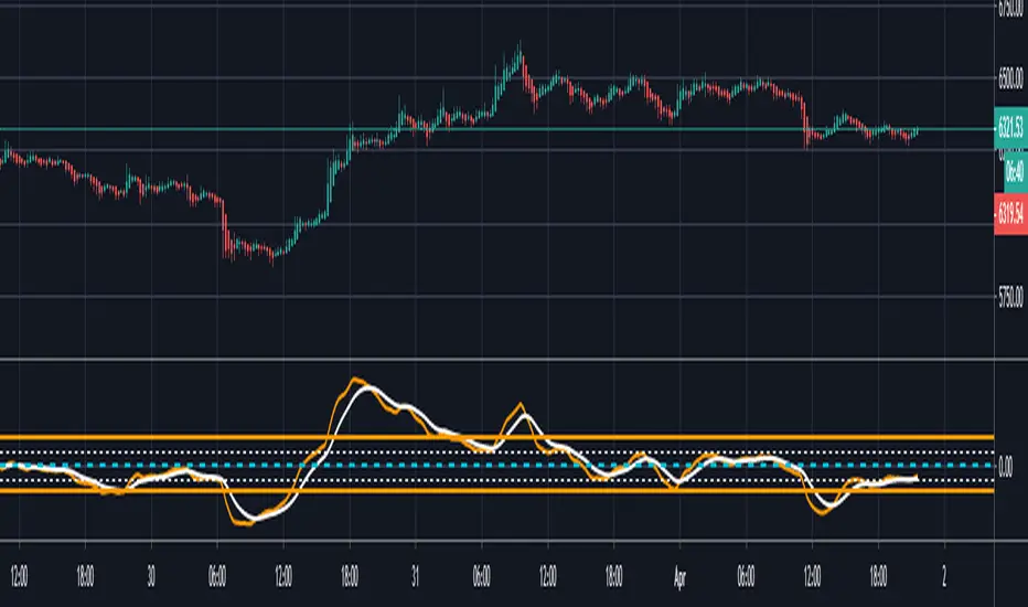
Easy Directional Movement IndexNothing more than a graphical tweak for the integrated Directional movement index (DMI). The purpose is to make the reading of the DMI easier and more immediate.
The area between DI+ and DI- is filled, and the indicator's range in divided into 4 sections, each of them representing a different price tendency:
- When ADX line is inside the red colored area (0-25), the market is in a ranging phase.
- When inside the aqua colored area (25-50), there is a trend.
- When inside the blue colored area (50-75), there is a strong trend
- When inside the navy colored area (75-100), there is an extremely strong trend.
However keep in mind that these are default levels that may be not always significant. You can change them from the script settings as you prefer, to better tweak your analysis.
Please support my work and follow me if you like my scripts. Many more of them are coming in the future.
@Bezzus
ابحث في النصوص البرمجية عن "英国央行降息25个基点"

Ichimoku with Correct DisplacementThe default Ichimoku Cloud by TradingView is strange. The kumo is only displaced 25 periods forward, and the chikou is displaced 25 periods back. This is because TradingView had the correct value for displacement (26), but they decided to subtract this displacement by 1 when actually drawing the kumo and add 1 when drawing the chikou. This script fixes this and allows for easier customization of each line in the Ichimoku.

MACD At Scales with AlertsI use the horizontal scale lines on the MACD indicator as part of my scalping strategy along with other indicators like RSI/EMA and Market Cipher B when trading BTC
I am looking for a cross above or below the 12.5 and 25 horizontal scale lines, along with lining up other indicators
I set my alerts on the 5 min TF and look to the 15 and 30 min TF's for further confirmation.
I have find the scale lines to be very useful for visual reference of the crosses, above/below 25 lines is mostly a safer trade, crosses above/below 12.5 lines can have more risk, crosses between 0 baseline and 12.5 can have a higher return but have much more risk.
Don't ever use just this indicator by itself, you must always have at least 2 indicators running
This is an example of the TF's not lining up, so a entry here would be high risk
This is an example of the TF's lining up, so a entry here would be less risk
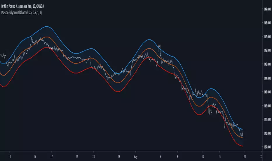
Pseudo Polynomial ChannelIntroduction
Back when i started using pine i made a script called periodic channel who aimed to rescale an average correlated sine wave to the price...don't worked very well. So i tried to fix problems induced by the indicator without much success, i had to redo it from scratch while abandoning the idea of rescaling correlated smooth functions to the price, at that time i also received requests regarding polynomial channel, some plateformes included this indicator, this led me to the idea to estimate it in order to both respond to the periodic channel problems and the requests i received, i have tried many many things and recently i tweaked a linear extrapolation to have an approximation.
Linear Extrapolation To Pseudo Polynomial Regression
I could be wrong but a polynomial regression must use constant parameters in order to provide a really smooth output, at least constant for a set of time. The moving averages forms (Savitzky-Golay moving average) who smooth polynomials across a window to the data don't have such smoothness, so how to estimate a polynomial regression while having a parameter providing control over the smoothness, a response to this is by using a recursive linear extrapolation. I posted a linear extrapolation indicator long ago, i used the same formula while adding a function to morph the output and the input in the form of :
morph * output + (1-morph) * input
How can this provide an estimate of a polynomial regression ? Well i'm not even sure myself but if you use the output as input (morph = 1) for the linear extrapolation function you should get a rough estimate of a line, this is what i thought at first and it proved to be right
Based on this observation i thought that it would be possible to get polynomial results by lowering morph, and as expected it worked well but showed a periodic pattern, this is why i smooth k in line 10.
0.9 for morph work well, higher values create sometimes smoother results but damage heavily the estimation.
Parameters
Morph have been introduced earlier, it control the amount of output and input the linear extrapolation should process, lower values create rougher but more stables results, if you see that the estimation is going nuts lower morph or change length, also lower length if you increase morph .
High overshoot, morph to 0.8 can help have a better estimation at the cost of less smoothness.
Length control the indicator smoothing, this parameter differ heavily from other filters, therefore low values can create mid/long term smoothing, it can also depend on which market instrument you are applying it, so there are no fixed optimal length.
Mult control how spread the bands are, to do so mult multiply the cumulative mean error, you can change this error measurement by anything you want like standard deviation/atr/range but take into account that you may create a separate parameter to control the error instead of length . Mult can be a float and like length can have different optimal values depending on the market the indicator is applied to.
Flatten do exactly what is name imply, it flatten the overall output to have a better estimation, can be a float. The result is less smooth.
Flatten = 2
More Exemples
BTCUSD length = 25 and mult = 4
XPDUSD length = 25 and mult = 1
ALPHABET length = 6 and morph = 0.99
Conclusion
I tried to estimate a polynomial channel by using recursion in the linear extrapolation function. This build is way more stable than the periodic channel but its still a bit inaccurate in my opinion. I hope this code can still help someone build something really nice, if so share your results :)
I apologize for those expecting a legit polynomial channel build but i really don't know how to do that, as i said parameters for the regression must be constants, i hope it still fine :)
Thanks for reading !
Modified Gann HiLo ActivatorIntroduction
The gann hilo activator is a trend indicator developed by Robert Krausz published into W. D. Gann Treasure Discovered: Simple Trading Plans for Stocks & Commodities . This indicator crate a trailing stop aiming to show the direction of the trend.
This indicator is fairly easy to compute and dont require lot of skills to understand. First we calculate the simple moving average of both price high and price low, when the close price is higher than the moving average of the price high the indicator return the moving average of the price low, else the indicator return the moving average of the price high if the close price is lower than the moving average of the price low.
My indicator add a different calculation method in order to avoid whipsaw trades as well as adding significance to the moving average length. A Median method has been added to provide more robustness.
The Indicator
The indicator is a simple trailing stop aiming to show the direction of the trend. The indicator use a different source instead of the price high/low for its calculation. The first method is the "SMA" method which like the classic hilo indicator use a simple moving average for the calculation of the indicator.
Sma Method with length = 25
The "Median" use a moving median instead of a simple moving average, this provide more robustness.
Median Method with length = 25
The shape is less curved and the indicator can sometimes avoid whipsaw with high's length periods.
Mult Parameter
The mult parameter is a parameter set to be lower or equal to 1 and greater or equal to 0. High values allow the indicator to be far from the price thus avoiding whipsaw trades, lower ones lower the distance from the price. A mult parameter of 0.1 approximate the original hilo indicator.
In blue the indicator with mult = 0.1 and in radical red the original hilo activator.
Conclusion
The modifications allow more control over the indicator as well as adding more robustness while the original one is destined to fail when market price is more complex.
Thanks for reading :)
For any questions/suggestions feel free to pm me

Average Candle LengthThis script is designed to show you the average candle size in pips (wick to wick) for however many bars you choose (20 is default).
The idea is that if the average candle size for the last 20 bars is, let's say 25, you would probably not want to set your stop loss less than 25 because it is more likely to get hit.
if you find this script helpful, tips and donations are always appreciated (venmo @rick-munoz) :)

Future Least Squares Moving Average//+------------------------------------------------------------------+
// | Future Least Squares Moving Average |
// | 未来予測LSMA |
// | Ver.1.0 |
// | Copyright Sakura |
//+------------------------------------------------------------------+
//LSMAは一時回帰直線の現在地の点の集合であるということは、未来の点を使えば未来を描けるはずというアホなことを無理やり考えました。
//結論はうまくいかなかったですので、パラメーターをいじって誤魔化しという結果に。
//それでも、先に書いてますので急激な価格変動に対処できる訳もなくといった感じになっています。
//displacementは一目に合わせたいので26固定の方向でとしたいところですが厳しいですね。
//
//設定例
//SMA(25)≒FLSMA(25,7,13)
//SMA(50)≒FLSMA(50,13,26)
//SMA(75)≒FLSMA(75,20,26)

How to automate this strategy for free using a chrome extension.Hey everyone,
Recently we developed a chrome extension for automating TradingView strategies using the alerts they provide. Initially we were charging a monthly fee for the extension, but we have now decided to make it FREE for everyone. So to display the power of automating strategies via TradingView, we figured we would also provide a profitable strategy along with the custom alert script and commands for the alerts so you can easily cut and paste to begin trading for profit while you sleep.
Step 1:
You are going to need to download the Chrome Extension called AutoView. You can get the extension for free by following this link: bit.ly ( I had to shorten the link as it contains Google and TV automatically converts it to a symbol)
Step 2: Go to your chrome extension page, and under the new extension you'll see a "settings" button. In the setting you will have to connect and give permission to the exchange 1broker allowing the extension to place your orders automatically when triggered by an alert.
Step 3: Setup the strategy and custom script for the alerts in TradingView. The attached script is the strategy, you can play with the settings yourself to try and get better numbers/performance if you please.
This following script is for the custom alerts:
//@version=2
study("4All-Alert", shorttitle="Alerts")
src = close
len = input(4, minval=1, title="Length")
up = rma(max(change(src), 0), len)
down = rma(-min(change(src), 0), len)
rsi = down == 0 ? 100 : up == 0 ? 0 : 100 - (100 / (1 + up / down))
rsin = input(5)
sn = 100 - rsin
ln = 0 + rsin
short = crossover(rsi, sn) ? 1 : 0
long = crossunder(rsi, ln) ? 1 : 0
plot(long, "Long", color=green)
plot(short, "Short", color=red)
Now that you have the extension installed, the custom strategy and alert scripts in place, you simply need to create the alerts.
To get the alerts to communicate with the extension properly, there is a specific syntax that you will need to put in the message of the alert. You can find more details about the syntax here : gist.github.com
For this specific strategy, I use the Alerts script, long/short greater than 0.9 on close.
In the message for a long place this as your message:
Long
c=order b=short
c=position b=short l=200 t=market
b=long q=0.01 l=200 t=market tp=13 sl=25
and for the short...
Short
c=order b=long
c=position b=long l=200 t=market
b=short q=0.01 l=200 t=market tp=13 sl=25
If you'll notice in my above messages, compared to the strategy my tp and sl (take profit and stop loss) vary by a few pips. This is to cover the market opens and spread on 1broker. You can change the tp and sl in the strategy to the above and see that the overall profit will not vary much at all.
I hope this all makes sense and it is enough to not only make some people money, but to show the power of coming up with your own strategy and automating it using TradingView alerts and the free Chrome Extension AutoView.
ps. I highly recommend upgrading your TradingView account so you have access to back testing and multiple alerts.
There is really no reason you won't cover the cost and then some on a monthly basis using the tools provided.
Best of luck and happy trading.
Note: The extension currently allows for automation on 2 exchanges; 1broker and Okcoin. If you do not have accounts there, we'd appreciate you signing up using our referral links.
www.okcoin.com
1broker.com

dhruv private 91400//@version=5
//
VERSION = '7.9-X'// 2024.3.20
strategy(
'LE VAN DO® - Swing Signals & Overlays Private™ 7.9-X',
shorttitle = 'LE VAN DO® - Swing Signals & Overlays Private™ 7.9-X' + VERSION,
overlay = true,
explicit_plot_zorder = true,
pyramiding = 0,
default_qty_type = strategy.percent_of_equity,
default_qty_value = 50,
calc_on_every_tick = false,
process_orders_on_close = true,
max_bars_back = 500,
initial_capital = 5000,
commission_type = strategy.commission.percent,
commission_value = 0.02,
max_lines_count = 500
)
//Truncate Function
truncate(number, decimals) =>
factor = math.pow(10, decimals)
int(number * factor) / factor
//
// === INPUTS ===
TPSType = input.string('Trailing', 'What TPS should be taken : ', options = )
setupType = input.string('Open/Close', title='What Trading Setup should be taken : ', options= )
scolor = input(true, title='Show coloured Bars to indicate Trend?')
almaRibbon = input(false, title='Enable Ribbon?')
//tradeType = input.string('BOTH', title='What trades should be taken : ', options= )
// === /INPUTS ===
// Display the probabilities in a table
//text01_ = str.tostring(timeframe.multiplier * intRes, '####')
//t = timenow + math.round(ta.change(time) * 25)
//var label lab01 = na
//label.delete(lab01)
//lab01 := label.new(t, close, text=text01_, style=label.style_label_left, yloc=yloc.price, xloc=xloc.bar_time, textalign=text.align_left, textcolor=color.white)
// Constants colours that include fully non-transparent option.
green100 = #008000FF
lime100 = #66bb6a
red100 = #f7525f
blue100 = #0000FFFF
aqua100 = #00FFFFFF
darkred100 = #8B0000FF
gray100 = #808080FF
/////////////////////////////////////////////
// Create non-repainting security function
rp_security(_symbol, _res, _src) =>
request.security(_symbol, _res, _src )
//
f_tfInMinutes() =>
_tfInMinutes = timeframe.period == '1' ? '3' : timeframe.period == '3' ? '5' : timeframe.period == '5' ? '15' : timeframe.period == '15' ? '30' : timeframe.period == '30' ? '60' : timeframe.period == '60' ? '240' : 'D'
_tfInMinutes
my_time1 = f_tfInMinutes()
tfmult = 18 //input.int(18, "Input Timeframe Multiplier")
f_resInMinutes() =>
_resInMinutes = timeframe.multiplier * (
timeframe.isseconds ? 1. / 60. :
timeframe.isminutes ? 1. :
timeframe.isdaily ? 1440. :
timeframe.isweekly ? 10080. :
timeframe.ismonthly ? 43800. : na)
my_time = str.tostring(f_resInMinutes()*tfmult)
useSource = close //input.string('Close', 'What Source to be used?', options = )
enableFilter = input(true, "Enable Backtesting Range Filtering")
fromDate = input.time(timestamp("01 Jan 2023 00:00 +0300"), "Start Date")
toDate = input.time(timestamp("31 Dec 2099 00:00 +0300"), "End Date")
tradeDateIsAllowed = not enableFilter or (time >= fromDate and time <= toDate)
filter1 = 'Filter with Atr'
filter2 = 'Filter with RSI'
filter3 = 'Atr or RSI'
filter4 = 'Atr and RSI'
filter5 = 'No Filtering'
filter6 = 'Entry Only in sideways market(By ATR or RSI)'
filter7 = 'Entry Only in sideways market(By ATR and RSI)'
typefilter = input.string(filter5, title='Sideways Filtering Input', options= , group='Strategy Options')
RSI = truncate(ta.rsi(close, input.int(7, group='RSI Filterring')), 2)
toplimitrsi = input.int(45, title='TOP Limit', group='RSI Filterring')
botlimitrsi = input.int(10, title='BOT Limit', group='RSI Filterring')
//ST = input.bool(true, title='Show Supertrend?', group='Supertrend Indicator')
//period = input.int(1440, group='Supertrend Indicator')
//mult = input.float(2.612, group='Supertrend Indicator')
atrfiltLen = 5 //input.int(5, minval=1, title='atr Length', group='Sideways Filtering Input')
atrMaType = 'EMA' //input.string('EMA', options= , group='Sideways Filtering Input', title='atr Moving Average Type')
atrMaLen = 5 //input.int(5, minval=1, title='atr MA Length', group='Sideways Filtering Input')
//filtering
atra = request.security(syminfo.tickerid, '', ta.atr(atrfiltLen))
atrMa = atrMaType == 'EM' ? ta.ema(atra, atrMaLen) : ta.sma(atra, atrMaLen)
updm = ta.change(high)
downdm = -ta.change(low)
plusdm = na(updm) ? na : updm > downdm and updm > 0 ? updm : 0
minusdm = na(downdm) ? na : downdm > updm and downdm > 0 ? downdm : 0
cndSidwayss1 = atra >= atrMa
cndSidwayss2 = RSI > toplimitrsi or RSI < botlimitrsi
cndSidways = cndSidwayss1 or cndSidwayss2
cndSidways1 = cndSidwayss1 and cndSidwayss2
Sidwayss1 = atra <= atrMa
Sidwayss2 = RSI < toplimitrsi and RSI > botlimitrsi
Sidways = Sidwayss1 or Sidwayss2
Sidways1 = Sidwayss1 and Sidwayss2
trendType = typefilter == filter1 ? cndSidwayss1 : typefilter == filter2 ? cndSidwayss2 : typefilter == filter3 ? cndSidways : typefilter == filter4 ? cndSidways1 : typefilter == filter5 ? RSI > 0 : typefilter == filter6 ? Sidways : typefilter == filter7 ? Sidways1 : na
// === /INPUTS ===
tf = my_time //input('15')
r = ticker.heikinashi(syminfo.tickerid)
openSeriesAlt = request.security(r, tf, open, lookahead=barmerge.lookahead_on)
closeSeriesAlt = request.security(r, tf, close, lookahead=barmerge.lookahead_on)
//openP = plot(almaRibbon ? openSeriesAlt : na, color=color.new(color.lime, 0), linewidth=3)
//closeP = plot(almaRibbon ? closeSeriesAlt : na, color=color.new(color.red, 0), linewidth=3)
BUYOC = ta.crossover(closeSeriesAlt, openSeriesAlt) and setupType == "Open/Close" and trendType
SELLOC = ta.crossunder(closeSeriesAlt, openSeriesAlt) and setupType == "Open/Close" and trendType
//strategy.entry('sell', direction=strategy.short, qty=trade_size, comment='sell', when=sel_entry)
//strategy.entry('buy', direction=strategy.long, qty=trade_size, comment='buy', when=buy_entry)
//trendColour = closeSeriesAlt > openSeriesAlt ? color.green : color.red
//bcolour = closeSeriesAlt > openSeriesAlt ? lime100 : red100
//barcolor(scolor ? bcolour : na, title='Bar Colours')
//closeP = plot(almaRibbon ? closeSeriesAlt : na, title='Close Series', color=color.new(trendColour, 20), linewidth=2, style=plot.style_line)
//openP = plot(almaRibbon ? openSeriesAlt : na, title='Open Series', color=color.new(trendColour, 20), linewidth=2, style=plot.style_line)
//fill(closeP, openP, color=color.new(trendColour, 80))
//
//rt = input(true, title="ATR Based REnko is the Default, UnCheck to use Traditional ATR?")
atrLen = 3 //input.int(3, title="RENKO_ATR", group = "Renko Settings")
isATR = true //input.bool(true, title="RENKO_USE_RENKO_ATR", group = "Renko Settings")
tradLen1 = 1000 //input.int(1000, title="RENKO_TRADITIONAL", group = "Renko Settings")
//Code to be implemented in V2
//mul = input(1, "Number Of minticks")
//value = mul * syminfo.mintick
tradLen = tradLen1 * 1
param = isATR ? ticker.renko(syminfo.tickerid, "ATR", atrLen) : ticker.renko(syminfo.tickerid, "Traditional", tradLen)
renko_close = request.security(param, my_time, close, lookahead=barmerge.lookahead_on)
renko_open = request.security(param, my_time, open, lookahead=barmerge.lookahead_on)
//============================================
//Sniper------------------------------------------------------------------------------------------------------------------------------------- // Signal 2
//============================================
//============================================
//EMA_CROSS-------------------------------------------------------------------------------------------------------------------------------- // Signal 4
//============================================
EMA1_length=input.int(2, "EMA1_length", group = "Renko Settings")
EMA2_length=input.int(10, "EMA2_length", group = "Renko Settings")
a = ta.ema(renko_close, EMA1_length)
b = ta.ema(renko_close, EMA2_length)
//BUY = ta.cross(a, b) and a > b and renko_open < renko_close
//SELL = ta.cross(a, b) and a < b and renko_close < renko_open
///////////////////////////////
// Determine long and short conditions
BUYR = ta.crossover(a, b) and setupType == "Renko" and trendType
SELLR = ta.crossunder(a, b) and setupType == "Renko" and trendType
sel_color = setupType == "Open/Close" ? closeSeriesAlt < openSeriesAlt : setupType == "Renko" ? renko_close < renko_open : na
buy_color = setupType == "Open/Close" ? closeSeriesAlt > openSeriesAlt : setupType == "Renko" ? renko_close > renko_open : na
sel_entry = setupType == "Open/Close" ? SELLOC : setupType == "Renko" ? SELLR : na
buy_entry = setupType == "Open/Close" ? BUYOC : setupType == "Renko" ? BUYR : na
trendColour = buy_color ? color.green : color.red
bcolour = buy_color ? lime100 : red100
barcolor(scolor ? bcolour : na, title='Bar Colours')
p11=plot(almaRibbon and setupType == "Open/Close" ? closeSeriesAlt : almaRibbon and setupType == "Renko" ? renko_close : na, style=plot.style_circles, linewidth=1, color=color.new(trendColour, 80), title="RENKO_1")
p22=plot(almaRibbon and setupType == "Open/Close" ? openSeriesAlt : almaRibbon and setupType == "Renko" ? renko_open : na, style=plot.style_circles, linewidth=1, color=color.new(trendColour, 80), title="RENKO_2")
fill(p11, p22, color=color.new(trendColour, 50), title="RENKO_fill")
//
lxTrigger = false
sxTrigger = false
leTrigger = buy_entry
seTrigger = sel_entry
// === /ALERT conditions.
buy = leTrigger //ta.crossover(closeSeriesAlt, openSeriesAlt)
sell = seTrigger //ta.crossunder(closeSeriesAlt, openSeriesAlt)
varip wasLong = false
varip wasShort = false
if barstate.isconfirmed
wasLong := false
else
if buy
wasLong := true
if barstate.isconfirmed
wasShort := false
else
if sell
wasShort := true
plotshape(wasLong, color = color.yellow)
plotshape(wasShort, color = color.yellow)
//plotshape(almaRibbon ? buy : na, title = "Buy", text = 'Buy', style = shape.labelup, location = location.belowbar, color= #39ff14, textcolor = #FFFFFF, size = size.tiny)
//plotshape(almaRibbon ? sell : na, title = "Exit", text = 'Exit', style = shape.labeldown, location = location.abovebar, color= #ff1100, textcolor = #FFFFFF, size = size.tiny)
// === STRATEGY ===
i_alert_txt_entry_long = "Short Exit" //input.text_area(defval = "Short Exit", title = "Long Entry Message", group = "Alerts")
i_alert_txt_exit_long = "Long Exit" //input.text_area(defval = "Long Exit", title = "Long Exit Message", group = "Alerts")
i_alert_txt_entry_short = "Go Short" //input.text_area(defval = "Go Short", title = "Short Entry Message", group = "Alerts")
i_alert_txt_exit_short = "Go Long" //input.text_area(defval = "Go Long", title = "Short Exit Message", group = "Alerts")
// Entries and Exits with TP/SL
//tradeType
if buy and TPSType == "Trailing" and tradeDateIsAllowed
strategy.close("Short" , alert_message = i_alert_txt_exit_short)
strategy.entry("Long" , strategy.long , alert_message = i_alert_txt_entry_long)
if sell and TPSType == "Trailing" and tradeDateIsAllowed
strategy.close("Long" , alert_message = i_alert_txt_exit_long)
strategy.entry("Short" , strategy.short, alert_message = i_alert_txt_entry_short)
//tradeType
if buy and TPSType == "Options" and tradeDateIsAllowed
// strategy.close("Short" , alert_message = i_alert_txt_exit_short)
strategy.entry("Long" , strategy.long , alert_message = i_alert_txt_entry_long)
if sell and TPSType == "Options" and tradeDateIsAllowed
strategy.close("Long" , alert_message = i_alert_txt_exit_long)
// strategy.entry("Short" , strategy.short, alert_message = i_alert_txt_entry_short)
G_RISK = '■ ' + 'Risk Management'
//#region ———— <↓↓↓ G_RISK ↓↓↓> {
//ATR SL Settings
atrLength = 20 //input.int(20, minval=1, title='ATR Length')
profitFactor = 2.5 //input(2.5, title='Take Profit Factor')
stopFactor = 1 //input(1.0, title='Stop Loss Factor')
// Calculate ATR
tpatrValue = ta.atr(atrLength)
// Calculate take profit and stop loss levels for buy signals
takeProfit1_buy = 1 * profitFactor * tpatrValue //close + profitFactor * atrValue
takeProfit2_buy = 2 * profitFactor * tpatrValue //close + 2 * profitFactor * atrValue
takeProfit3_buy = 3 * profitFactor * tpatrValue //close + 3 * profitFactor * atrValue
stopLoss_buy = close - takeProfit1_buy //stopFactor * tpatrValue
// Calculate take profit and stop loss levels for sell signals
takeProfit1_sell = 1 * profitFactor * tpatrValue //close - profitFactor * atrValue
takeProfit2_sell = 2 * profitFactor * tpatrValue //close - 2 * profitFactor * atrValue
takeProfit3_sell = 3 * profitFactor * tpatrValue //close - 3 * profitFactor * atrValue
stopLoss_sell = close + takeProfit1_sell //stopFactor * tpatrValue
// ———————————
//Tooltip
T_LVL = '(%) Exit Level'
T_QTY = '(%) Adjust trade exit volume'
T_MSG = 'Paste JSON message for your bot'
//Webhook Message
O_LEMSG = 'Long Entry'
O_LXMSGSL = 'Long SL'
O_LXMSGTP1 = 'Long TP1'
O_LXMSGTP2 = 'Long TP2'
O_LXMSGTP3 = 'Long TP3'
O_LXMSG = 'Long Exit'
O_SEMSG = 'Short Entry'
O_SXMSGSL = 'Short SL'
O_SXMSGA = 'Short TP1'
O_SXMSGB = 'Short TP2'
O_SXMSGC = 'Short TP3'
O_SXMSGX = 'Short Exit'
// on whole pips) for forex currency pairs.
pip_size = syminfo.mintick * (syminfo.type == "forex" ? 10 : 1)
// On the last historical bar, show the instrument's pip size
//if barstate.islastconfirmedhistory
// label.new(x=bar_index + 2, y=close, style=label.style_label_left,
// color=color.navy, textcolor=color.white, size=size.large,
// text=syminfo.ticker + "'s pip size is:\n" +
// str.tostring(pip_size))
// ——————————— | | | Line length guide |
i_lxLvlTP1 = leTrigger ? takeProfit1_buy : seTrigger ? takeProfit1_sell : na //input.float (1, 'Level TP1' , group = G_RISK, tooltip = T_LVL)
i_lxQtyTP1 = input.float (50, 'Qty TP1' , group = G_RISK, tooltip = T_QTY)
i_lxLvlTP2 = leTrigger ? takeProfit2_buy : seTrigger ? takeProfit2_sell : na //input.float (1.5, 'Level TP2' , group = G_RISK, tooltip = T_LVL)
i_lxQtyTP2 = input.float (30, 'Qty TP2' , group = G_RISK, tooltip = T_QTY)
i_lxLvlTP3 = leTrigger ? takeProfit3_buy : seTrigger ? takeProfit3_sell : na //input.float (2, 'Level TP3' , group = G_RISK, tooltip = T_LVL)
i_lxQtyTP3 = input.float (20, 'Qty TP3' , group = G_RISK, tooltip = T_QTY)
i_lxLvlSL = leTrigger ? takeProfit1_buy : seTrigger ? takeProfit1_sell : na //input.float (0.5, 'Stop Loss' , group = G_RISK, tooltip = T_LVL)
i_sxLvlTP1 = i_lxLvlTP1
i_sxQtyTP1 = i_lxQtyTP1
i_sxLvlTP2 = i_lxLvlTP2
i_sxQtyTP2 = i_lxQtyTP2
i_sxLvlTP3 = i_lxLvlTP3
i_sxQtyTP3 = i_lxQtyTP3
i_sxLvlSL = i_lxLvlSL
G_MSG = '■ ' + 'Webhook Message'
i_leMsg = O_LEMSG //input.string (O_LEMSG ,'Long Entry' , group = G_MSG, tooltip = T_MSG)
i_lxMsgSL = O_LXMSGSL //input.string (O_LXMSGSL ,'Long SL' , group = G_MSG, tooltip = T_MSG)
i_lxMsgTP1 = O_LXMSGTP1 //input.string (O_LXMSGTP1,'Long TP1' , group = G_MSG, tooltip = T_MSG)
i_lxMsgTP2 = O_LXMSGTP2 //input.string (O_LXMSGTP2,'Long TP2' , group = G_MSG, tooltip = T_MSG)
i_lxMsgTP3 = O_LXMSGTP3 //input.string (O_LXMSGTP3,'Long TP3' , group = G_MSG, tooltip = T_MSG)
i_lxMsg = O_LXMSG //input.string (O_LXMSG ,'Long Exit' , group = G_MSG, tooltip = T_MSG)
i_seMsg = O_SEMSG //input.string (O_SEMSG ,'Short Entry' , group = G_MSG, tooltip = T_MSG)
i_sxMsgSL = O_SXMSGSL //input.string (O_SXMSGSL ,'Short SL' , group = G_MSG, tooltip = T_MSG)
i_sxMsgTP1 = O_SXMSGA //input.string (O_SXMSGA ,'Short TP1' , group = G_MSG, tooltip = T_MSG)
i_sxMsgTP2 = O_SXMSGB //input.string (O_SXMSGB ,'Short TP2' , group = G_MSG, tooltip = T_MSG)
i_sxMsgTP3 = O_SXMSGC //input.string (O_SXMSGC ,'Short TP3' , group = G_MSG, tooltip = T_MSG)
i_sxMsg = O_SXMSGX //input.string (O_SXMSGX ,'Short Exit' , group = G_MSG, tooltip = T_MSG)
i_src = close
G_DISPLAY = 'Display'
//
i_alertOn = true //input.bool (true, 'Alert Labels On/Off' , group = G_DISPLAY)
i_barColOn = true //input.bool (true, 'Bar Color On/Off' , group = G_DISPLAY)
// ———————————
// @function Calculate the Take Profit line, and the crossover or crossunder
f_tp(_condition, _conditionValue, _leTrigger, _seTrigger, _src, _lxLvlTP, _sxLvlTP)=>
var float _tpLine = 0.0
_topLvl = _src + _lxLvlTP //TPSType == "Fixed %" ? _src + (_src * (_lxLvlTP / 100)) : _src + _lxLvlTP
_botLvl = _src - _lxLvlTP //TPSType == "Fixed %" ? _src - (_src * (_sxLvlTP / 100)) : _src - _sxLvlTP
_tpLine := _condition != _conditionValue and _leTrigger ? _topLvl :
_condition != -_conditionValue and _seTrigger ? _botLvl :
nz(_tpLine )
// @function Similar to "ta.crossover" or "ta.crossunder"
f_cross(_scr1, _scr2, _over)=>
_cross = _over ? _scr1 > _scr2 and _scr1 < _scr2 :
_scr1 < _scr2 and _scr1 > _scr2
// ———————————
//
var float condition = 0.0
var float slLine = 0.0
var float entryLine = 0.0
//
entryLine := leTrigger and condition <= 0.0 ? close :
seTrigger and condition >= 0.0 ? close : nz(entryLine )
//
slTopLvl = TPSType == "Fixed %" ? i_src + (i_src * (i_lxLvlSL / 100)) : i_src + i_lxLvlSL
slBotLvl = TPSType == "Fixed %" ? i_src - (i_src * (i_sxLvlSL / 100)) : i_src - i_lxLvlSL
slLine := condition <= 0.0 and leTrigger ? slBotLvl :
condition >= 0.0 and seTrigger ? slTopLvl : nz(slLine )
slLong = f_cross(low, slLine, false)
slShort = f_cross(high, slLine, true )
//
= f_tp(condition, 1.2,leTrigger, seTrigger, i_src, i_lxLvlTP3, i_sxLvlTP3)
= f_tp(condition, 1.1,leTrigger, seTrigger, i_src, i_lxLvlTP2, i_sxLvlTP2)
= f_tp(condition, 1.0,leTrigger, seTrigger, i_src, i_lxLvlTP1, i_sxLvlTP1)
tp3Long = f_cross(high, tp3Line, true )
tp3Short = f_cross(low, tp3Line, false)
tp2Long = f_cross(high, tp2Line, true )
tp2Short = f_cross(low, tp2Line, false)
tp1Long = f_cross(high, tp1Line, true )
tp1Short = f_cross(low, tp1Line, false)
switch
leTrigger and condition <= 0.0 => condition := 1.0
seTrigger and condition >= 0.0 => condition := -1.0
tp3Long and condition == 1.2 => condition := 1.3
tp3Short and condition == -1.2 => condition := -1.3
tp2Long and condition == 1.1 => condition := 1.2
tp2Short and condition == -1.1 => condition := -1.2
tp1Long and condition == 1.0 => condition := 1.1
tp1Short and condition == -1.0 => condition := -1.1
slLong and condition >= 1.0 => condition := 0.0
slShort and condition <= -1.0 => condition := 0.0
lxTrigger and condition >= 1.0 => condition := 0.0
sxTrigger and condition <= -1.0 => condition := 0.0
longE = leTrigger and condition <= 0.0 and condition == 1.0
shortE = seTrigger and condition >= 0.0 and condition == -1.0
longX = lxTrigger and condition >= 1.0 and condition == 0.0
shortX = sxTrigger and condition <= -1.0 and condition == 0.0
longSL = slLong and condition >= 1.0 and condition == 0.0
shortSL = slShort and condition <= -1.0 and condition == 0.0
longTP3 = tp3Long and condition == 1.2 and condition == 1.3
shortTP3 = tp3Short and condition == -1.2 and condition == -1.3
longTP2 = tp2Long and condition == 1.1 and condition == 1.2
shortTP2 = tp2Short and condition == -1.1 and condition == -1.2
longTP1 = tp1Long and condition == 1.0 and condition == 1.1
shortTP1 = tp1Short and condition == -1.0 and condition == -1.1
// ——————————— {
//
if strategy.position_size <= 0 and longE and TPSType == "ATR" and tradeDateIsAllowed
strategy.entry( 'Long', strategy.long, alert_message = i_leMsg, comment = 'LE')
if strategy.position_size > 0 and condition == 1.0 and TPSType == "ATR" and tradeDateIsAllowed
strategy.exit( id = 'LXTP1', from_entry = 'Long', qty_percent = i_lxQtyTP1, limit = tp1Line, stop = slLine, comment_profit = 'LXTP1', comment_loss = 'SL', alert_profit = i_lxMsgTP1, alert_loss = i_lxMsgSL)
if strategy.position_size > 0 and condition == 1.1 and TPSType == "ATR" and tradeDateIsAllowed
strategy.exit( id = 'LXTP2', from_entry = 'Long', qty_percent = i_lxQtyTP2, limit = tp2Line, stop = slLine, comment_profit = 'LXTP2', comment_loss = 'SL', alert_profit = i_lxMsgTP2, alert_loss = i_lxMsgSL)
if strategy.position_size > 0 and condition == 1.2 and TPSType == "ATR" and tradeDateIsAllowed
strategy.exit( id = 'LXTP3', from_entry = 'Long', qty_percent = i_lxQtyTP3, limit = tp3Line, stop = slLine, comment_profit = 'LXTP3', comment_loss = 'SL', alert_profit = i_lxMsgTP3, alert_loss = i_lxMsgSL)
if longX and tradeDateIsAllowed
strategy.close( 'Long', alert_message = i_lxMsg, comment = 'LX')
//
if strategy.position_size >= 0 and shortE and TPSType == "ATR" and tradeDateIsAllowed
strategy.entry( 'Short', strategy.short, alert_message = i_leMsg, comment = 'SE')
if strategy.position_size < 0 and condition == -1.0 and TPSType == "ATR" and tradeDateIsAllowed
strategy.exit( id = 'SXTP1', from_entry = 'Short', qty_percent = i_sxQtyTP1, limit = tp1Line, stop = slLine, comment_profit = 'SXTP1', comment_loss = 'SL', alert_profit = i_sxMsgTP1, alert_loss = i_sxMsgSL)
if strategy.position_size < 0 and condition == -1.1 and TPSType == "ATR" and tradeDateIsAllowed
strategy.exit( id = 'SXTP2', from_entry = 'Short', qty_percent = i_sxQtyTP2, limit = tp2Line, stop = slLine, comment_profit = 'SXTP2', comment_loss = 'SL', alert_profit = i_sxMsgTP2, alert_loss = i_sxMsgSL)
if strategy.position_size < 0 and condition == -1.2 and TPSType == "ATR" and tradeDateIsAllowed
strategy.exit( id = 'SXTP3', from_entry = 'Short', qty_percent = i_sxQtyTP3, limit = tp3Line, stop = slLine, comment_profit = 'SXTP3', comment_loss = 'SL', alert_profit = i_sxMsgTP3, alert_loss = i_sxMsgSL)
if shortX and tradeDateIsAllowed
strategy.close( 'Short', alert_message = i_sxMsg, comment = 'SX')
// ———————————
c_tp = leTrigger or seTrigger ? na :
condition == 0.0 ? na : color.green
c_entry = leTrigger or seTrigger ? na :
condition == 0.0 ? na : color.blue
c_sl = leTrigger or seTrigger ? na :
condition == 0.0 ? na : color.red
p_tp1Line = plot ( condition == 1.0 or condition == -1.0 ? tp1Line : na, title = "TP Line 1", color = c_tp, linewidth = 1, style = plot.style_linebr)
p_tp2Line = plot ( condition == 1.0 or condition == -1.0 or condition == 1.1 or condition == -1.1 ? tp2Line : na, title = "TP Line 2", color = c_tp, linewidth = 1, style = plot.style_linebr)
p_tp3Line = plot ( condition == 1.0 or condition == -1.0 or condition == 1.1 or condition == -1.1 or condition == 1.2 or condition == -1.2 ? tp3Line : na, title = "TP Line 3", color = c_tp, linewidth = 1, style = plot.style_linebr)
p_entryLine = plot ( condition >= 1.0 or condition <= -1.0 ? entryLine : na, title = "Entry Line", color = c_entry, linewidth = 1, style = plot.style_linebr)
p_slLine = plot ( condition == 1.0 or condition == -1.0 or condition == 1.1 or condition == -1.1 or condition == 1.2 or condition == -1.2 ? slLine : na, title = "SL Line", color = c_sl, linewidth = 1, style = plot.style_linebr)
//fill( p_tp3Line, p_entryLine, color = leTrigger or seTrigger ? na :color.new(color.green, 90))
fill( p_entryLine, p_slLine, color = leTrigger or seTrigger ? na :color.new(color.red, 90))
//
plotshape( i_alertOn and longE, title = 'Long', text = 'Long', textcolor = color.white, color = color.green, style = shape.labelup, size = size.tiny, location = location.belowbar)
plotshape( i_alertOn and shortE, title = 'Short', text = 'Short', textcolor = color.white, color = color.red, style = shape.labeldown, size = size.tiny, location = location.abovebar)
plotshape( i_alertOn and (longX or shortX) ? close : na, title = 'Close', text = 'Close', textcolor = color.white, color = color.gray, style = shape.labelup, size = size.tiny, location = location.absolute)
l_tp = i_alertOn and (longTP1 or shortTP1) ? close : na
plotshape( l_tp, title = "TP1 Cross", text = "TP1", textcolor = color.white, color = #ec407a, style = shape.labelup, size = size.tiny, location = location.absolute)
plotshape( i_alertOn and (longTP2 or shortTP2) ? close : na, title = "TP2 Cross", text = "TP2", textcolor = color.white, color = #ec407a, style = shape.labelup, size = size.tiny, location = location.absolute)
plotshape( i_alertOn and (longTP3 or shortTP3) ? close : na, title = "TP3 Cross", text = "TP3", textcolor = color.white, color = #ec407a, style = shape.labelup, size = size.tiny, location = location.absolute)
plotshape( i_alertOn and (longSL or shortSL) ? close : na, title = "SL Cross", text = "SL", textcolor = color.white, color = color.maroon, style = shape.labelup, size = size.tiny, location = location.absolute)
//
plot( na, title = "─── ───", editable = false, display = display.data_window)
plot( condition, title = "condition", editable = false, display = display.data_window)
plot( strategy.position_size * 100, title = ".position_size", editable = false, display = display.data_window)
//#endregion }
// ——————————— <↑↑↑ G_RISK ↑↑↑>
//#region ———— <↓↓↓ G_SCRIPT02 ↓↓↓> {
// @function Queues a new element in an array and de-queues its first element.
f_qDq(_array, _val) =>
array.push(_array, _val)
_return = array.shift(_array)
_return
var line a_slLine = array.new_line(1)
var line a_entryLine = array.new_line(1)
var line a_tp3Line = array.new_line(1)
var line a_tp2Line = array.new_line(1)
var line a_tp1Line = array.new_line(1)
var label a_slLabel = array.new_label(1)
var label a_tp3label = array.new_label(1)
var label a_tp2label = array.new_label(1)
var label a_tp1label = array.new_label(1)
var label a_entryLabel = array.new_label(1)
newEntry = longE or shortE
entryIndex = 1
entryIndex := newEntry ? bar_index : nz(entryIndex )
lasTrade = bar_index >= entryIndex
l_right = 10
if TPSType == "ATR"
line.delete( f_qDq(a_slLine, line.new( entryIndex, slLine, last_bar_index + l_right, slLine, style = line.style_solid, color = c_sl)))
if TPSType == "ATR"
line.delete( f_qDq(a_entryLine, line.new( entryIndex, entryLine, last_bar_index + l_right, entryLine, style = line.style_solid, color = color.blue)))
if TPSType == "ATR"
line.delete( f_qDq(a_tp3Line, line.new( entryIndex, tp3Line, last_bar_index + l_right, tp3Line, style = line.style_solid, color = c_tp)))
if TPSType == "ATR"
line.delete( f_qDq(a_tp2Line, line.new( entryIndex, tp2Line, last_bar_index + l_right, tp2Line, style = line.style_solid, color = c_tp)))
if TPSType == "ATR"
line.delete( f_qDq(a_tp1Line, line.new( entryIndex, tp1Line, last_bar_index + l_right, tp1Line, style = line.style_solid, color = c_tp)))
if TPSType == "ATR"
label.delete( f_qDq(a_slLabel, label.new( last_bar_index + l_right, slLine, 'SL: ' + str.tostring(slLine, '##.###'), style = label.style_label_left, textcolor = color.white, color = c_sl)))
if TPSType == "ATR"
label.delete( f_qDq(a_entryLabel, label.new( last_bar_index + l_right, entryLine, 'Entry: ' + str.tostring(entryLine, '##.###'), style = label.style_label_left, textcolor = color.white, color = color.blue)))
if TPSType == "ATR"
label.delete( f_qDq(a_tp3label, label.new( last_bar_index + l_right, tp3Line, 'TP3: ' + str.tostring(tp3Line, '##.###') + " - Target Pips : - " + str.tostring(longE ? tp3Line - entryLine : entryLine - tp3Line, "#.##"), style = label.style_label_left, textcolor = color.white, color = c_tp)))
if TPSType == "ATR"
label.delete( f_qDq(a_tp2label, label.new( last_bar_index + l_right, tp2Line, 'TP2: ' + str.tostring(tp2Line, '##.###'), style = label.style_label_left, textcolor = color.white, color = c_tp)))
if TPSType == "ATR"
label.delete( f_qDq(a_tp1label, label.new( last_bar_index + l_right, tp1Line, 'TP1: ' + str.tostring(tp1Line, '##.###'), style = label.style_label_left, textcolor = color.white, color = c_tp)))
//#endregion }
// ——————————— <↑↑↑ G_SCRIPT02 ↑↑↑>
c_barCol = close > open ? color.rgb(120, 9, 139) : color.rgb(69, 155, 225)
barcolor(
i_barColOn ? c_barCol : na)
// ———————————
//
if longE or shortE or longX or shortX
alert(message = 'Any Alert', freq = alert.freq_once_per_bar_close)
if longE
alert(message = 'Long Entry', freq = alert.freq_once_per_bar_close)
if shortE
alert(message = 'Short Entry', freq = alert.freq_once_per_bar_close)
if longX
alert(message = 'Long Exit', freq = alert.freq_once_per_bar_close)
if shortX
alert(message = 'Short Exit', freq = alert.freq_once_per_bar_close)
//#endregion }
// ——————————— <↑↑↑ G_SCRIPT03 ↑↑↑>
// This source code is subject to the terms of the Mozilla Public License 2.0 at mozilla.org
// © TraderHalai
// This script was born out of my quest to be able to display strategy back test statistics on charts to allow for easier backtesting on devices that do not natively support backtest engine (such as mobile phones, when I am backtesting from away from my computer). There are already a few good ones on TradingView, but most / many are too complicated for my needs.
//
//Found an excellent display backtest engine by 'The Art of Trading'. This script is a snippet of his hard work, with some very minor tweaks and changes. Much respect to the original author.
//
//Full credit to the original author of this script. It can be found here: www.tradingview.com
//
// This script can be copied and airlifted onto existing strategy scripts of your own, and integrates out of the box without implementation of additional functions. I've also added Max Runup, Average Win and Average Loss per trade to the orignal script.
//
//Will look to add in more performance metrics in future, as I further develop this script.
//
//Feel free to use this display panel in your scripts and strategies.
//Thanks and enjoy! :)
//@version=5
//strategy("Strategy BackTest Display Statistics - TraderHalai", overlay=true, default_qty_value= 5, default_qty_type = strategy.percent_of_equity, initial_capital=10000, commission_type=strategy.commission.percent, commission_value=0.1)
//DEMO basic strategy - Use your own strategy here - Jaws Mean Reversion from my profile used here
//source = input(title = "Source", defval = close)
///////////////////////////// --- BEGIN TESTER CODE --- ////////////////////////
// COPY below into your strategy to enable display
////////////////////////////////////////////////////////////////////////////////
// Declare performance tracking variables
drawTester = input.bool(false, "Strategy Performance", group='Dashboards', inline="Show Dashboards")
var balance = strategy.initial_capital
var drawdown = 0.0
var maxDrawdown = 0.0
var maxBalance = 0.0
var totalWins = 0
var totalLoss = 0
// Prepare stats table
var table testTable = table.new(position.top_right, 5, 2, border_width=1)
f_fillCell(_table, _column, _row, _title, _value, _bgcolor, _txtcolor) =>
_cellText = _title + "\n" + _value
table.cell(_table, _column, _row, _cellText, bgcolor=_bgcolor, text_color=_txtcolor)
// Custom function to truncate (cut) excess decimal places
//truncate(_number, _decimalPlaces) =>
// _factor = math.pow(10, _decimalPlaces)
// int(_number * _factor) / _factor
// Draw stats table
var bgcolor = color.new(color.black,0)
if drawTester and tradeDateIsAllowed
if barstate.islastconfirmedhistory
// Update table
dollarReturn = strategy.netprofit
f_fillCell(testTable, 0, 0, "Total Trades:", str.tostring(strategy.closedtrades), bgcolor, color.white)
f_fillCell(testTable, 0, 1, "Win Rate:", str.tostring(truncate((strategy.wintrades/strategy.closedtrades)*100,2)) + "%", bgcolor, color.white)
f_fillCell(testTable, 1, 0, "Starting:", "$" + str.tostring(strategy.initial_capital), bgcolor, color.white)
f_fillCell(testTable, 1, 1, "Ending:", "$" + str.tostring(truncate(strategy.initial_capital + strategy.netprofit,2)), bgcolor, color.white)
f_fillCell(testTable, 2, 0, "Avg Win:", "$"+ str.tostring(truncate(strategy.grossprofit / strategy.wintrades, 2)), bgcolor, color.white)
f_fillCell(testTable, 2, 1, "Avg Loss:", "$"+ str.tostring(truncate(strategy.grossloss / strategy.losstrades, 2)), bgcolor, color.white)
f_fillCell(testTable, 3, 0, "Profit Factor:", str.tostring(truncate(strategy.grossprofit / strategy.grossloss,2)), strategy.grossprofit > strategy.grossloss ? color.green : color.red, color.white)
f_fillCell(testTable, 3, 1, "Max Runup:", str.tostring(truncate(strategy.max_runup, 2 )), bgcolor, color.white)
f_fillCell(testTable, 4, 0, "Return:", (dollarReturn > 0 ? "+" : "") + str.tostring(truncate((dollarReturn / strategy.initial_capital)*100,2)) + "%", dollarReturn > 0 ? color.green : color.red, color.white)
f_fillCell(testTable, 4, 1, "Max DD:", str.tostring(truncate((strategy.max_drawdown / strategy.equity) * 100 ,2)) + "%", color.red, color.white)
// --- END TESTER CODE --- ///////////////
// This Pine Script™ code is subject to the terms of the Mozilla Public License 2.0 at mozilla.org
// © niceGear68734
//@version=5
//strategy("Table to filter trades per day", overlay=true, use_bar_magnifier = true, initial_capital = 5000, calc_on_every_tick = true, calc_on_order_fills = true, commission_type = strategy.commission.cash_per_contract)
//~ ___________________________________________________________________________
//~ !!!!!!!!!!!!!!!!!!!!!!!!!!!!!!!!!!!!!!!!!!!!!!!!!!!!!!!!!!!!!!!!!!!!!!!!!!!
//~ !!!!!!!!!!!!!!!_________________ START _________________!!!!!!!!!!!!!!!!!
i_showweeklyPerformance = input.bool(false, 'Weekly Performance', group='Dashboards', inline="Show Dashboards")
//__________________________ User Inputs ___________________________________
var const string g_table = "Table Settings"
i_table_pos = "Top Left" //input.string(defval = "Top Left", title = "Position", options = , group = g_table, inline = "1", tooltip = "It sets the location of the table")
i_text_size = "Normal" //input.string(defval = "Normal", title = "Set the size of text", options = , tooltip = "This option is used to change the size of the text in the table")
var const string g_general = "General Settings"
i_check_open_close = "Opened" //input.string("Opened", "Check when the trade :", , group = g_general, tooltip = "This parameter defines what to check for. If opened is selected, the results will show the trades that opened on that day. If closed is selected, the results will show the trades that closed on that day")
i_timezone = "Exchange" //input.string("Exchange", title = "Set the Timezone", options = , group = g_general, tooltip = "You can use this setting whenever you want to change the time that the trade has closed/opened")
//~_____________________________ Switches ___________________________________
table_pos = switch i_table_pos
"Bottom Right" => position.bottom_right
"Bottom Left" => position.bottom_left
"Top Right" => position.top_right
"Top Left" => position.top_left
timezone_setting = i_timezone == "Exchange" ? syminfo.timezone : i_timezone
text_size = switch i_text_size
"Small" => size.small
"Normal" => size.normal
"Large" => size.large
//__________________________ Array Declaration _____________________________
var string t_column_names = array.from( "", "Sun", "Mon", "Tue", "Wed", "Thur", "Fri", "Sat") // Columns header names
var string t_row_names = array.from("", "Total Trades", "Loss", "Win", "Win Rate" ) // Rows header names
var t_column_size = array.size(t_column_names)
var t_row_size = array.size(t_row_names)
var string a_closed_trades = array.new_string() // Save the total number of trades
var string a_loss_trades = array.new_string() // Save the number of losing trades
var string a_win_trades = array.new_string() // Save the number of winning trades
var _a_day_week = array.new_int() // Save the day of the week to split data
// __________________________ Custom Functions ________________________________
//~ create a counter so that it gives a number to strategy.closed_trades.entry_time(counter)
var trade_number = -1
if strategy.closedtrades > strategy.closedtrades
trade_number += 1
f_strategy_closedtrades_hour() =>
switch
i_check_open_close =="Closed" => dayofweek(strategy.closedtrades.exit_time(trade_number), timezone_setting)
i_check_open_close =="Opened" => dayofweek(strategy.closedtrades.entry_time(trade_number), timezone_setting)
f_data(_i) =>
var _closed_trades = 0
var _loss_trades = 0
var _win_trades = 0
var _txt_closed_trades = ""
var _txt_loss_trades = ""
var _txt_win_trades = ""
if strategy.closedtrades > strategy.closedtrades and f_strategy_closedtrades_hour() == _i
_closed_trades += 1
_txt_closed_trades := str.tostring(_closed_trades)
if strategy.losstrades > strategy.losstrades and f_strategy_closedtrades_hour() == _i
_loss_trades += 1
_txt_loss_trades := str.tostring(_loss_trades)
if strategy.wintrades > strategy.wintrades and f_strategy_closedtrades_hour() == _i
_win_trades += 1
_txt_win_trades := str.tostring(_win_trades)
//__________________________
var string array1 = array.new_string(5)
var string array2 = array.new_string(5)
var string array3 = array.new_string(5)
var string array4 = array.new_string(5)
var string array5 = array.new_string(5)
var string array6 = array.new_string(5)
var string array7 = array.new_string(5)
f_pass_data_to_array(_i, _array) =>
= f_data(_i)
array.set(_array,1 , cl)
array.set(_array,2,loss)
array.set(_array,3,win)
if cl != ""
array.set(_array,4,str.tostring(str.tonumber(win) / str.tonumber(cl) * 100 , "##") + " %")
if cl != "" and win == ""
array.set(_array,4,"0 %")
for i = 1 to 7
switch
i == 1 => f_pass_data_to_array(i,array1)
i == 2 => f_pass_data_to_array(i,array2)
i == 3 => f_pass_data_to_array(i,array3)
i == 4 => f_pass_data_to_array(i,array4)
i == 5 => f_pass_data_to_array(i,array5)
i == 6 => f_pass_data_to_array(i,array6)
i == 7 => f_pass_data_to_array(i,array7)
f_retrieve_data_to_table(_i, _j) =>
switch
_i == 1 => array.get(array1, _j)
_i == 2 => array.get(array2, _j)
_i == 3 => array.get(array3, _j)
_i == 4 => array.get(array4, _j)
_i == 5 => array.get(array5, _j)
_i == 6 => array.get(array6, _j)
_i == 7 => array.get(array7, _j)
//~ ___________________________ Create Table ________________________________
create_table(_col, _row, _txt) =>
var table _tbl = table.new(position = table_pos, columns = t_column_size , rows = t_row_size, border_width=1)
color _color = _row == 0 or _col == 0 ? color.rgb(3, 62, 106) : color.rgb(2, 81, 155)
table.cell(_tbl, _col, _row, _txt, bgcolor = _color, text_color = color.white, text_size = text_size)
//~___________________________ Fill With Data _______________________________
if barstate.islastconfirmedhistory and i_showweeklyPerformance and tradeDateIsAllowed
for i = 0 to t_column_size - 1 by 1
for j = 0 to t_row_size - 1 by 1
_txt = ""
if i >= 0 and j == 0
_txt := array.get(t_column_names, i)
if j >= 0 and i == 0
_txt := array.get(t_row_names, j)
if i >= 1 and j >= 1 and j <= 5
_txt := f_retrieve_data_to_table( i , j)
create_table(i ,j , _txt)
//~ ___________________________ Notice ______________________________________
if timeframe.in_seconds() > timeframe.in_seconds("D")
x = table.new(position.middle_center,1,1,color.aqua)
table.cell_set_text(x,0,0,"Please select lower timeframes (Daily or lower)")
//~ !!!!!!!!!!!!!!!_________________ STOP _________________!!!!!!!!!!!!!!!!!!
//~ !!!!!!!!!!!!!!!!!!!!!!!!!!!!!!!!!!!!!!!!!!!!!!!!!!!!!!!!!!!!!!!!!!!!!!!!!!!
//~ ___________________________________________________________________________
// Global Dashboard Variables
// ░░░░░░░░░░░░░░░░░░░░░░░░░░░░░░░░░░░░░░░░░░░░░░░░░░░░░░░░░░░░░░░░░░░░░░░░░░░░░░░░░░░░░░░░░░░░░░░░░░░░░░░░░░░░░░░░░░░░░░░░░░░░░░░░░░░░░░░░░░░░░░░░░░
// Dashboard Table Text Size
i_tableTextSize = "Normal" //input.string(title="Dashboard Size", defval="Normal", options= , group="Dashboards")
table_text_size(s) =>
switch s
"Auto" => size.auto
"Huge" => size.huge
"Large" => size.large
"Normal" => size.normal
"Small" => size.small
=> size.tiny
tableTextSize = table_text_size(i_tableTextSize)
// Monthly Table Performance Dashboard By @QuantNomad
// ░░░░░░░░░░░░░░░░░░░░░░░░░░░░░░░░░░░░░░░░░░░░░░░░░░░░░░░░░░░░░░░░░░░░░░░░░░░░░░░░░░░░░░░░░░░░░░░░░░░░░░░░░░░░░░░░░░░░░░░░░░░░░░░░░░░░░░░░░░░░░░░░░░
i_showMonthlyPerformance = input.bool(false, 'Monthly Performance', group='Dashboards', inline="Show Dashboards")
i_monthlyReturnPercision = 2
if i_showMonthlyPerformance and tradeDateIsAllowed
new_month = month(time) != month(time )
new_year = year(time) != year(time )
eq = strategy.equity
bar_pnl = eq / eq - 1
cur_month_pnl = 0.0
cur_year_pnl = 0.0
// Current Monthly P&L;
cur_month_pnl := new_month ? 0.0 :
(1 + cur_month_pnl ) * (1 + bar_pnl) - 1
// Current Yearly P&L;
cur_year_pnl := new_year ? 0.0 :
(1 + cur_year_pnl ) * (1 + bar_pnl) - 1
// Arrays to store Yearly and Monthly P&Ls;
var month_pnl = array.new_float(0)
var month_time = array.new_int(0)
var year_pnl = array.new_float(0)
var year_time = array.new_int(0)
last_computed = false
if (not na(cur_month_pnl ) and (new_month or barstate.islastconfirmedhistory))
if (last_computed )
array.pop(month_pnl)
array.pop(month_time)
array.push(month_pnl , cur_month_pnl )
array.push(month_time, time )
if (not na(cur_year_pnl ) and (new_year or barstate.islastconfirmedhistory))
if (last_computed )
array.pop(year_pnl)
array.pop(year_time)
array.push(year_pnl , cur_year_pnl )
array.push(year_time, time )
last_computed := barstate.islastconfirmedhistory ? true : nz(last_computed )
// Monthly P&L; Table
var monthly_table = table(na)
if (barstate.islastconfirmedhistory)
monthly_table := table.new(position.bottom_right, columns = 14, rows = array.size(year_pnl) + 1, border_width = 1)
table.cell(monthly_table, 0, 0, "", bgcolor = #cccccc, text_size=tableTextSize)
table.cell(monthly_table, 1, 0, "Jan", bgcolor = #cccccc, text_size=tableTextSize)
table.cell(monthly_table, 2, 0, "Feb", bgcolor = #cccccc, text_size=tableTextSize)
table.cell(monthly_table, 3, 0, "Mar", bgcolor = #cccccc, text_size=tableTextSize)
table.cell(monthly_table, 4, 0, "Apr", bgcolor = #cccccc, text_size=tableTextSize)
table.cell(monthly_table, 5, 0, "May", bgcolor = #cccccc, text_size=tableTextSize)
table.cell(monthly_table, 6, 0, "Jun", bgcolor = #cccccc, text_size=tableTextSize)
table.cell(monthly_table, 7, 0, "Jul", bgcolor = #cccccc, text_size=tableTextSize)
table.cell(monthly_table, 8, 0, "Aug", bgcolor = #cccccc, text_size=tableTextSize)
table.cell(monthly_table, 9, 0, "Sep", bgcolor = #cccccc, text_size=tableTextSize)
table.cell(monthly_table, 10, 0, "Oct", bgcolor = #cccccc, text_size=tableTextSize)
table.cell(monthly_table, 11, 0, "Nov", bgcolor = #cccccc, text_size=tableTextSize)
table.cell(monthly_table, 12, 0, "Dec", bgcolor = #cccccc, text_size=tableTextSize)
table.cell(monthly_table, 13, 0, "Year", bgcolor = #999999, text_size=tableTextSize)
for yi = 0 to array.size(year_pnl) - 1
table.cell(monthly_table, 0, yi + 1, str.tostring(year(array.get(year_time, yi))), bgcolor = #cccccc, text_size=tableTextSize)
y_color = array.get(year_pnl, yi) > 0 ? color.new(color.teal, transp = 40) : color.new(color.gray, transp = 40)
table.cell(monthly_table, 13, yi + 1, str.tostring(math.round(array.get(year_pnl, yi) * 100, i_monthlyReturnPercision)), bgcolor = y_color, text_color=color.new(color.white, 0),text_size=tableTextSize)
for mi = 0 to array.size(month_time) - 1
m_row = year(array.get(month_time, mi)) - year(array.get(year_time, 0)) + 1
m_col = month(array.get(month_time, mi))
m_color = array.get(month_pnl, mi) > 0 ? color.new(color.teal, transp = 40) : color.new(color.maroon, transp = 40)
table.cell(monthly_table, m_col, m_row, str.tostring(math.round(array.get(month_pnl, mi) * 100, i_monthlyReturnPercision)), bgcolor = m_color, text_color=color.new(color.white, 0), text_size=tableTextSize)
hide = timeframe.isintraday
// Input for EMA period
emaPeriod = 48 //input.int(48, title="EMA Period")
emaPeriod2 = 2 //input.int(2, title="EME Period 2")
emaPeriod3 = 21 //input.int(21, title="EMA Period")
// Input to toggle EMA Cloud
showcloud = input.bool(false, title="Plot EMA?", group='EMA & ATR', inline="Show EMA's & ATR")
useHTF = input.bool(true, title = "Use Higher Time Frame?")
matimeframe = useHTF ? my_time1 : ''
// EMA calculations
ema = request.security(syminfo.tickerid, matimeframe, ta.ema(close, emaPeriod))
ema2 = request.security(syminfo.tickerid, matimeframe, ta.ema(close,emaPeriod2))
ema3 = request.security(syminfo.tickerid, matimeframe,ta.ema(close, emaPeriod3))
emaColor = close > ema3 ? color.new(color.rgb(56, 142, 60, 63), 50) : color.new(color.rgb(147, 40, 51, 38), 50)
// Plotting EMA's
// plot_ema1 = plot(hide ? ema : na, style=plot.style_line, color=color.new(color.rgb(255, 255, 255, 100), 50), title="EMA", linewidth=2)
// plot_ema2 = plot(hide ? ema2 : na, style=plot.style_line, color=color.new(color.rgb(255, 255, 255, 100), 50), title="EMA", linewidth=1)
// plot_ema3 = plot(ema3, style=plot.style_line, color=emaColor, title="EMA", linewidth=1)
// EMA Cloud
cloudColor = ema2 > ema ? color.new(#0f8513, 80) : color.new(#a81414, 80)
cloudColor2 = ema2 > ema3 ? color.new(#0f8513, 50) : color.new(#a81414, 50)
cloudColor := showcloud ? cloudColor : na
// fill(plot_ema1, plot_ema2, color=cloudColor, title="EMA Cloud")
// fill(plot_ema3, plot_ema2, color=cloudColor, title="EMA Cloud")
/////////////////////////////////////////////////////////////// © BackQuant ///////////////////////////////////////////////////////////////
// This Pine Script™ code is subject to the terms of the Mozilla Public License 2.0 at mozilla.org
// © BackQuant
import TradingView/ta/4 as ta
//@version=5
//indicator(
// title="DEMA Adjusted Average True Range ",
// shorttitle = "DEMA ATR ",
// overlay=true,
// timeframe="",
// timeframe_gaps=true
// )
// Define User Inputs
simple bool showAtr = input.bool(false, "Plot Dema?", group='EMA & ATR', inline="Show EMA's & ATR")
simple bool haCandles = true //input.bool(true, "Use HA Candles?")
simple int periodDema = 7 //input.int(7, "Dema Period", group = "Dema Atr")
series float sourceDema = close //input.source(close, "Calculation Source", group = "Dema Atr")
simple int periodAtr = 14 //input.int(14, "Period", group = "Dema Atr")
simple float factorAtr = 1.7 //input.float(1.7, "Factor", step = 0.01, group = "Dema Atr")
simple color longColour = #66bb6a
simple color shortColour = #f23645
/////////////////////////////////////////////////////////////// © BackQuant ///////////////////////////////////////////////////////////////
// Use HA Candles?
heikinashi_close = request.security(
symbol = ticker.heikinashi(syminfo.tickerid),
timeframe = timeframe.period,
expression = close,
gaps = barmerge.gaps_off,
lookahead = barmerge.lookahead_on
)
var series float source = close
if haCandles == true
source := heikinashi_close
if haCandles == false
source := sourceDema
/////////////////////////////////////////////////////////////// © BackQuant ///////////////////////////////////////////////////////////////
// Function
DemaAtrWithBands(periodDema, source, lookback, atrFactor)=>
ema1 = ta.ema(source, periodDema)
ema2 = ta.ema(ema1, periodDema)
demaOut = 2 * ema1 - ema2
atr = ta.atr(lookback)
trueRange = atr * atrFactor
DemaAtr = demaOut
DemaAtr := nz(DemaAtr , DemaAtr)
trueRangeUpper = demaOut + trueRange
trueRangeLower = demaOut - trueRange
if trueRangeLower > DemaAtr
DemaAtr := trueRangeLower
if trueRangeUpper < DemaAtr
DemaAtr := trueRangeUpper
DemaAtr
// Function Out
DemaAtr = DemaAtrWithBands(periodDema, source, periodAtr, factorAtr)
/////////////////////////////////////////////////////////////// © BackQuant ///////////////////////////////////////////////////////////////
// Conditions
DemaAtrLong = DemaAtr > DemaAtr
DemaAtrShort = DemaAtr < DemaAtr
// Colour Condtions
var color Trendcolor = #ffffff
if DemaAtrLong
Trendcolor := longColour
if DemaAtrShort
Trendcolor := shortColour
// Plotting
plot( showAtr ? DemaAtr : na, "ATR", color=Trendcolor, linewidth = 2 )
import DevLucem/ZigLib/1 as ZigZag
////////
// Fetch Ingredients
//
// ////////
// // Bake it with a simple oven this time
= ZigZag.zigzag(low, high, Depth, Deviation, Backstep)
string nowPoint = ""
var float lastPoint = z1.price
if bool(ta.change(direction))
lastPoint := z1.price
// ////////
// // Let it Cool And Serve
line zz = na
label point = na
if repaint
zz := line.new(z1, z2, xloc.bar_time, extend? extend.right: extend.none, color.new(direction>0? upcolor: dncolor, lines), width=line_thick)
nowPoint := direction<0? (z2.pricelastPoint? "HH": "LH")
point := label.new(z2, nowPoint, xloc.bar_time, yloc.price,
color.new(direction<0? upcolor: dncolor, labels), direction>0? label.style_label_down: label.style_label_up, color.new(direction>0? upcolor: dncolor, labels), label_size)
if direction == direction
line.delete(zz )
label.delete(point )
else
line.set_extend(zz , extend.none)
else
if direction != direction
zz := line.new(z1 , z2 , xloc.bar_time, extend.none, color.new(direction>0? upcolor: dncolor, lines), width=line_thick)
nowPoint := direction <0? (z2.price lastPoint ? "HH": "LH")
point := label.new(z2 , nowPoint, xloc.bar_time, yloc.price,
color.new(direction <0? upcolor: dncolor, labels), direction >0? label.style_label_down: label.style_label_up, color.new(direction >0? upcolor: dncolor, labels), label_size)
bgcolor(direction<0? color.new(dncolor, background): color.new(upcolor, background), title='Direction Background', display = display.none)
plotarrow(direction, "direction", display=display.status_line)
// ////////
// // Declare Meal Was Sweet By Force
alertcondition(nowPoint == "HH" and z2.price != z2.price , "New Higher High", 'Zigzag on {{ticker}} higher higher high detected at {{time}}')
alertcondition(nowPoint == "LH" and z2.price != z2.price , "New Lower High", 'Zigzag on {{ticker}} higher lower high detected at {{time}}')
alertcondition(nowPoint == "HL" and z2.price != z2.price , "New Higher Low", 'Zigzag on {{ticker}} higher lower low detected at {{time}}')
alertcondition(nowPoint == "LL" and z2.price != z2.price , "New Lower Low", 'Zigzag on {{ticker}} lower low detected at {{time}}')
alertcondition(direction != direction , 'Direction Changed', 'Zigzag on {{ticker}} direction changed at {{time}}')
alertcondition(direction != direction and direction>0, 'Bullish Direction', 'Zigzag on {{ticker}} bullish direction at {{time}}')
alertcondition(direction != direction and direction<0, 'Bearish Direction', 'Zigzag on {{ticker}} bearish direction at {{time}}')
if direction != direction
alert((direction<0? "Bearish": "Bullish") + " Direction Final ", alert.freq_once_per_bar_close)
MSG = "MARKET STRUCTURE"
VBG = "VOLUMETRIC ORDER BLOCKS"
MST = "Limit market structure calculation to improve memory speed time"
SLT = " Limit swing structure to tot bars back"
IDT = " Start date of the internal structure"
CST = "Color candle based on trend detection system"
OBT = "Display internal buy and sell activity"
OBD = "Show Last number of orderblock"
OBMT = " Use Length to adjust cordinate of the orderblocks\n Use whole candle body"
_ ='
------------
–––––––––––––––––––––––––– INPUTS –––––––––––––––––––––––––––
------------ '//{
bool windowsis = input.bool(true, "Window", inline="kla", group=MSG)
int mswindow = input.int(5000, "", tooltip=MST,group=MSG, inline="kla", minval=1000)
bool showSwing = input.bool(true, "Swing", inline="scss", group=MSG)
int swingLimit = input.int(100, "", tooltip=SLT, inline="scss", group=MSG, minval=10, maxval=200)
color swingcssup = input.color(#f7525f, "", inline="scss", group=MSG)
color swingcssdn = input.color(#66bb6a, "", inline="scss", group=MSG)
bool showMapping = input.bool(false, "Mapping Structure", inline="mapping", group=MSG)
string mappingStyle = input.string("----", "", options= , inline="mapping", group=MSG)
color mappingcss = input.color(color.silver, "", tooltip="Display Mapping Structure", inline="mapping", group=MSG)
bool candlecss = input.bool(false, "Color Candles", tooltip=CST, group=MSG, inline="txt")
string mstext = input.string("Tiny", "", options= ,
inline="txt", group=MSG)
string msmode = input.string("Adjusted Points", "Algorithmic Logic", options=
, inline="node", group=MSG)
int mslen = input.int(5, "", inline="node", group=MSG, minval=2)
bool buildsweep = input.bool(true, "Build Sweep (x)", "Build sweep on market structure", "znc", MSG)
bool msbubble = input.bool(true, "Bubbles", tooltip="Display Circle Bubbles", inline="bubbles", group=MSG)
bool obshow = input.bool(true, "Show Last", tooltip=OBD, group=VBG, inline="obshow")
int oblast = input.int(5, "", group=VBG, inline="obshow", minval=0)
color obupcs = input.color(color.new(#089981, 90), "", inline="obshow", group=VBG)
color obdncs = input.color(color.new(#f23645, 90), "", inline="obshow", group=VBG)
bool obshowactivity = input.bool(true, "Show Buy/Sell Activity", inline="act", group=VBG, tooltip=OBT)
color obactup = input.color(color.new(#089981, 50), "", inline="act", group=VBG)
color obactdn = input.color(color.new(#f23645, 50), "", inline="act", group=VBG)
obshowbb = input.bool(false, "Show Breakers", inline="bb", group=VBG, tooltip="Display Breakers")
color bbup = input.color(color.new(#089981, 100), "", inline="bb", group=VBG)
color bbdn = input.color(color.new(#f23645, 100), "", inline="bb", group=VBG)
obmode = input.string("Length", "Construction", options= , tooltip=OBMT, inline="atr", group=VBG)
len = input.int(5, "", inline="atr", group=VBG, minval=1)
obmiti = input.string("Close", "Mitigation Method", options= ,
tooltip="Mitigation method for when to trigger order blocks", group=VBG)
obtxt = input.string("Normal", "Metric Size", options= ,
tooltip="Order block Metrics text size", inline="txt", group=VBG)
showmetric = input.bool(true, "Show Metrics", group=VBG)
showline = input.bool(true, "Show Mid-Line", group=VBG)
overlap = input.bool(true, "Hide Overlap", group=VBG, inline="ov")
wichlap = input.string("Recent", "", options= , inline="ov", group=VBG)
fvg_enable = input.bool(false, "", inline="1", group="FAIR VALUE GAP", tooltip="Display fair value gap")
what_fvg = input.string("FVG", "", inline="1", group="FAIR VALUE GAP", tooltip="Display fair value gap",
options= )
fvg_num = input.int(5, "Show Last", inline="1a", group="FAIR VALUE GAP", tooltip="Number of fvg to show", minval=0)
fvg_upcss = input.color(color.new(#089981, 80), "", inline="1", group="FAIR VALUE GAP")
fvg_dncss = input.color(color.new(#f23645, 80), "", inline="1", group="FAIR VALUE GAP")
fvgbbup = input.color(color.new(#089981, 100), "", inline="1", group="FAIR VALUE GAP")
fvgbbdn = input.color(color.new(#f23645, 100), "", inline="1", group="FAIR VALUE GAP")
fvg_src = input.string("Close", "Mitigation",
inline="3",
group="FAIR VALUE GAP",
tooltip=" Use the close of the body as trigger\n\n Use the extreme point of the body as trigger",
options= )
fvgthresh = input.float(0, "Threshold", tooltip="Filter out non significative FVG", group="FAIR VALUE GAP",
inline="asd", minval=0, maxval=2, step=0.1)
fvgoverlap = input.bool(true, "Hide Overlap", "Hide overlapping FVG", group="FAIR VALUE GAP")
fvgline = input.bool(true, "Show Mid-Line", group="FAIR VALUE GAP")
fvgextend = input.bool(false, "Extend FVG", group="FAIR VALUE GAP")
dispraid = input.bool(false, "Display Raids", inline="raid", group="FAIR VALUE GAP")
//}
_ ='
------------
–––––––––––––––––––––––––– UDT –––––––––––––––––––––––––––
------------ '//{
type hqlzone
box pbx
box ebx
box lbx
label plb
label elb
label lbl
type Zphl
line top
line bottom
label top_label
label bottom_label
bool stopcross
bool sbottomcross
bool itopcross
bool ibottomcross
string txtup
string txtdn
float topy
float bottomy
float topx
float bottomx
float tup
float tdn
int tupx
int tdnx
float itopy
float itopx
float ibottomy
float ibottomx
float uV
float dV
type entered
bool normal = false
bool breaker = false
type store
line ln
label lb
box bx
linefill lf
type structure
int zn
float zz
float bos
float choch
int loc
int temp
int trend
int start
float main
int xloc
bool upsweep
bool dnsweep
string txt = na
type drawms
int x1
int x2
float y
string txt
color css
string style
type ob
bool bull
float top
float btm
float avg
int loc
color css
float vol
int dir
int move
int blPOS
int brPOS
int xlocbl
int xlocbr
bool isbb = false
int bbloc
type FVG
float top = na
float btm = na
int loc = bar_index
bool isbb = false
int bbloc = na
bool israid = false
float raidy = na
int raidloc = na
int raidx2 = na
bool active = false
color raidcs = na
type SFP
float y
int loc
float ancor
type sfpbuildlbl
int x
float y
string style
color css
string txt
type sfpbuildline
int x1
int x2
float y
color css
float ancor
int loc
type equalbuild
int x1
float y1
int x2
float y2
color css
string style
type equalname
int x
float y
string txt
color css
string style
type ehl
float pt
int t
float pb
int b
type sellbuyside
float top
float btm
int loc
color css
string txt
float vol
type timer
bool start = false
int count = 0
//}
_ ='
------------
–––––––––––––––––––––––––– SETUP –––––––––––––––––––––––––––
------------ '//{
var store bin = store.new(
array.new< line >()
, array.new< label >()
, array.new< box >()
, array.new()
)
var entered blobenter = entered.new()
var entered brobenter = entered.new()
var entered blfvgenter = entered.new()
var entered brfvgenter = entered.new()
var entered blarea = entered.new()
var entered brarea = entered.new()
var timer lc = timer.new ()
if barstate.islast
for obj in bin.ln
obj.delete()
for obj in bin.lb
obj.delete()
for obj in bin.bx
obj.delete()
for obj in bin.lf
obj.delete()
bin.ln.clear()
bin.lb.clear()
bin.bx.clear()
bin.lf.clear()
invcol = #ffffff00
float atr = (ta.atr(200) / (5/len))
//}
_ ='
------------
–––––––––––––––––––––––––– UTILITY –––––––––––––––––––––––––––
------------ '//{
method txSz(string s) =>
out = switch s
"Tiny" => size.tiny
"Small" => size.small
"Normal" => size.normal
"Large" => size.large
"Huge" => size.huge
"Auto" => size.auto
out
method lstyle(string style) =>
out = switch style
'⎯⎯⎯⎯' => line.style_solid
'----' => line.style_dashed
'····' => line.style_dotted
ghl() => [high , low , close , open , close, open, high, low, high , low , ta.atr(200)]
method IDMIDX(bool use_max, int loc) =>
min = 99999999.
max = 0.
idx = 0
if use_max
for i = 0 to (bar_index - loc)
max := math.max(high , max)
min := max == high ? low : min
idx := max == high ? i : idx
else
for i = 0 to (bar_index - loc)
min := math.min(low , min)
max := min == low ? high : max
idx := min == low ? i : idx
idx
SFPData() => [high, high , high , low, low , low , close, volume, time, bar_index , time ]
SFPcords() =>
RealTF = barstate.isrealtime ? 0 : 1
= SFPData()
[h , h1 , h2 , l , l1 , l2 , c , v , t , n , t1 ]
method find(structure ms, bool use_max, bool sweep, bool useob) =>
min = 99999999.
max = 0.
idx = 0
if not sweep
if ((bar_index - ms.loc) - 1) > 0
if use_max
for i = 0 to (bar_index - ms.loc) - 1
max := math.max(high , max)
min := max == high ? low : min
idx := max == high ? i : idx
if useob
if high

ICT Smart Money - PremiumCME_MINI:NQ1!
✅ Detecting FVG boxes (green/red) for A+ setups
✅ When price taps back into the FVG, it triggers an entry
✅ Shows the position boxes (green profit zone, red SL zone)
✅ Calculates SL (25-35 points auto or fixed)
✅ Sets TP1, TP2, TP3 based on liquidity levels (swing highs/lows)
✅ Shows labels with entry price, SL in points, and TP levels with R:R

OsMA by A8/4 - Limited Edition🌟 **OsMA by A8/4 — The Ultimate Indicator for XAUUSD Trading** 🌟
An intelligent **automated system** designed exclusively for **gold trading**, equipped with everything you need in one tool 🔥
💡 **Key Features of OsMA by A8/4**
✅ **Auto Entry Signals**
Automatically detects trade opportunities using a **refined MACD Histogram formula** for enhanced accuracy.
Displays **LONG/SHORT arrows only on the first bar** to keep your chart clean and readable.
✅ **Auto Take Profit & Stop Loss System (Auto TP/SL)**
Once a signal appears, the system automatically sets:
* **TP1 = +15 USD**
* **TP2 = +25 USD**
* **SL = -10 USD**
These levels are displayed as **dashed lines** on the chart — clear and updated in real-time.
✅ **Smart DCA System (3 Orders)**
Works for both LONG and SHORT positions:
* **Order 1:** Entry upon signal confirmation (after candle close)
* **Order 2:** Entry at 5 USD below/above Order 1
* **Order 3:** Entry at another 5 USD below/above Order 2
The system automatically **calculates the average entry price** and **adjusts the SL** to -10 USD from the average cost.
This helps **spread risk** and **increase recovery potential** when prices rebound 💰
✅ **Specially Designed for XAUUSD Trading**
Compatible with both **Spot Gold** and **TFEX Gold Futures**.
Perfect for traders who value **clear, structured entry and exit strategies**.

MAOs🌟 **MAOs By A8/4 — The Ultimate Indicator for XAUUSD Trading** 🌟
An intelligent **automated system** designed exclusively for **gold trading**, equipped with everything you need in one tool 🔥
💡 **Key Features of MAOs By A8/4**
✅ **Auto Entry Signals**
Automatically detects trade opportunities using a **refined MACD Histogram formula** for enhanced accuracy.
Displays **LONG/SHORT arrows only on the first bar** to keep your chart clean and readable.
✅ **Auto Take Profit & Stop Loss System (Auto TP/SL)**
Once a signal appears, the system automatically sets:
* **TP1 = +15 USD**
* **TP2 = +25 USD**
* **SL = -10 USD**
These levels are displayed as **dashed lines** on the chart — clear and updated in real-time.
✅ **Smart DCA System (3 Orders)**
Works for both LONG and SHORT positions:
* **Order 1:** Entry upon signal confirmation (after candle close)
* **Order 2:** Entry at 5 USD below/above Order 1
* **Order 3:** Entry at another 5 USD below/above Order 2
The system automatically **calculates the average entry price** and **adjusts the SL** to -10 USD from the average cost.
This helps **spread risk** and **increase recovery potential** when prices rebound 💰
✅ **Specially Designed for XAUUSD Trading**
Compatible with both **Spot Gold** and **TFEX Gold Futures**.
Perfect for traders who value **clear, structured entry and exit strategies**.

Exhaustion Reversal Signals - ENHANCEDOverview
This is a reversal detection indicator that combines multiple technical analysis components to identify potential market turning points.
Core Components
1. Range Oscillator
Measures price deviation from a moving average (EMA/SMA) normalized by ATR
Values above +100 = bullish exhaustion zone
Values below -100 = bearish exhaustion zone
Detects momentum flattening (slope deceleration)
2. Stochastic Oscillator
Standard %K and %D with customizable parameters
Crossover detection (K crossing above/below D)
Oversold (<20) and Overbought (>80) zones
Momentum calculation (rate of change in K)
3. 🚀 Advanced Features
Early Detection System:
Identifies momentum exhaustion before confirmed crossovers
Detects when oscillator slope flattens (approaching zero)
Provides "advance warning" signals with relaxed thresholds
............................................................................................
Trend Filter:
50-period EMA for trend context
Three strength modes:
Soft: Allow all signals
Medium: Prefer trend-aligned signals
Strict: Only counter-trend reversals
Confidence Scoring (0-100%):
Oscillator extremity (30 pts)
Stochastic position (25 pts)
K-D divergence strength (20 pts)
Momentum alignment (15 pts)
Trend alignment (10 pts)
Minimum confidence threshold filtering
Visual Enhancements:
Dynamic background gradient (red→green based on oscillator)
Momentum bar coloring when slope flattens
Transparency adjustments based on momentum

Trend & Strength Detector TSDTrend Strength Detector (TSD)
*Objective Trend Quality Measurement for Educational Market Analysis*
Note: This mathematical framework is a proprietary quantitative model developed by Ario Pinelab, inspired by classical EMA, ADX, RSI and MACD principles, yet not documented in any public technical or academic publication.
## 🎯 Purpose & Design Philosophy
The ** Trend Strength Detector- TSD ** is an educational research tool that provides **quantitative measurement of trend quality** through two independent scoring systems (0-100 scale). It answers the analytical question: *"How strong and aligned is the current market trend environment?"*
This indicator is designed with a **modular, complementary approach** to work alongside various analysis methodologies, particularly pattern-based recognition systems.
## 🔗 Complementary Research Framework
### Designed to Work With Pattern Detection Systems
This indicator provides **environmental context measurement** that complements qualitative pattern recognition tools. It works particularly well alongside systems like:
- **RMBS Smart Detector - Multi-Factor Momentum System**
- Traditional chart pattern analyzers
- Any momentum-based pattern identification tools
🔍 **To find RMBS Smart Detector:**
- Search in TradingView Indicators Library: `" RMBS Smart Detector - Multi-Factor Momentum System"`
- Look for: *Multi-Factor Momentum System*
- By author: ` `
### Why This Complementary Approach?
**Trend Quality Measurement** (TSD - this tool) provides:
- ✅ Structural trend alignment (0-100 score)
- ✅ Momentum intensity levels (0-100 score)
- ✅ Environment classification (Strong/Moderate/Weak)
- 📌 **Answers:** *"HOW STRONG is the underlying trend environment?"*
### Educational Research Value
When used together in a research context, these tools enable systematic study of questions like:
- How do reversal patterns behave when Strength Score is above 70 vs below 30?
- Do continuation patterns in weakening environments (declining scores) show different characteristics?
- What is the correlation between high Alignment Scores and pattern "success rates"?
- Can environment classification help identify genuine trend initiation vs false starts?
⚠️ **Important Note:** Both tools are **independent and work standalone**. TSD provides value whether used alone or with other analysis methods. The relationship with RMBS (or any pattern tool) is **complementary for research purposes**, not dependent.
---
###Mathematical Foundation
##TSA Formula: scoring method developed by Ario
-Trend Model (0 – 100)
TAS = EMA Alignment (0–40) + Price Position (0–30) + Trend Consistency (0–30)
EMA Alignment checks EMA_fast vs EMA_slow vs EMA_trend structure.
Price Position evaluates if Close is above/below all EMAs.
Consistency = 3 × max(bullish,bearish bars within 10 candles).
-Strength Model (0 – 100)
Strength = ADX (0–50) + EMA Slope (0–25) + RSI (0–15) + MACD (0–10)
ADX measures trend energy; Slope shows EMA momentum %;
RSI assesses zone positioning; MACD confirms directional agreement.
Note: This formula represents a proprietary quantitative model by Ario_Pinelab, inspired by classical technical concepts but not published in any external reference.________________________________________
📊 Environment Classification
Based on Total Strength Score:
🟢 Strong Environment: Score ≥ 60
→ Well-defined momentum, clear directional bias
🟡 Moderate Environment: 40 ≤ Score < 60
→ Mixed signals, transitional conditions
🔴 Weak Environment: Score < 40
→ Ranging, choppy, low conviction movement
Color Coding:
• Green background: Strong (≥60)
• Yellow background: Moderate (40-59)
• Red background: Weak (<40)
________________________________________
📈 Visual Components
Main Chart Display
Score Labels (Top-Right Corner):
┌─────────────────────────────────┐
│ 📊 Alignment: 75 | Strength: 82 │
│ Environment: Strong 🟢 │
└─────────────────────────────────┘
Color-Coded Background:
• Environment strength visually indicated via background color
• Helps quick identification of market regime
• Customizable transparency (default: 90%)
Reference Lines:
• Dotted line at 60: Strong/Moderate threshold
• Dotted line at 40: Moderate/Weak threshold
• Mid-line at 50: Neutral reference
________________________________________
🔧 Customization Settings
Input Parameters
The best setting is the default mode.
🚫 Important Disclaimers & Limitations
What This Indicator IS:
✅ Educational measurement tool for trend quality research
✅ Quantitative assessment of current market environment
✅ Complementary analysis tool for pattern-based systems
✅ Historical data analyzer for systematic study
✅ Multi-factor scoring system based on technical calculations
What This Indicator IS NOT:
❌ NOT a trading system or signal generator
❌ NOT financial advice or trade recommendations
❌ NOT predictive of future price movements
❌ NOT a guarantee of pattern success/failure
❌ NOT a substitute for comprehensive risk management
________________________________________
Known Limitations
1. Lagging Nature:
⚠️ All components (EMA, ADX, RSI, MACD) are calculated
from historical price data
→ Scores reflect CURRENT and RECENT conditions
→ Cannot predict sudden reversals or black swan events
→ Trend measurements lag actual price turning points
2. Whipsaw Risk:
⚠️ In choppy/ranging markets, scores may fluctuate rapidly
→ Moderate zone (40-60) can see frequent transitions
→ Low timeframes more susceptible to noise
→ Consider higher timeframes for stable measurements
3. Component Conflicts:
⚠️ Individual components may disagree
→ Example: Strong ADX but weak RSI alignment
→ Scores average these conflicts (may hide nuance)
→ Check individual components for deeper insight
4. Not Predictive:
⚠️ High scores do NOT guarantee continuation
⚠️ Low scores do NOT guarantee reversal
→ Measurement ≠ Prediction
→ Use for CONTEXT, not SIGNALS
→ Combine with comprehensive analysis
________________________________________
Risk Acknowledgments
Market Risk:
• All trading involves substantial risk of loss
• Past performance (even systematic studies) does not guarantee future results
• No indicator, system, or methodology can eliminate market risk
Measurement Limitations:
• Scores are mathematical calculations, not market predictions
• Environmental classification is descriptive, not prescriptive
• Strong measurements can deteriorate rapidly without warning
Educational Purpose:
• This tool is designed for LEARNING about market structure
• Not designed, tested, or validated as a standalone trading system
• Any trading decisions are user’s sole responsibility
No Warranty:
• Indicator provided “as-is” for educational purposes
• No guarantee of accuracy, reliability, or profitability
• Users must verify calculations and apply critical thinking
Open Source
Full Pine Script code available for educational study and modification. Feedback and improvement suggestions welcome.
“All logic is presented for research and educational visualization.”
---
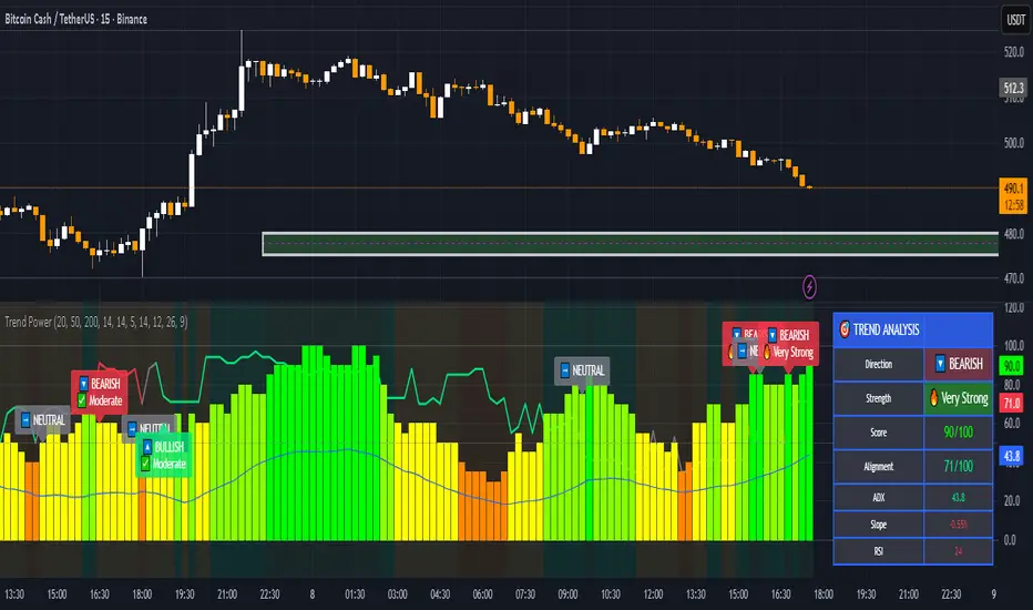
Power Balance ForecasterHey trader buddy! Remember the old IBM 5150 on Wall Street back in the 80s? :) Well, I wanted to pay tribute to it with this retro-style code when MS DOS and CRT screens were the cutting edge of technology...
Analysis of the balance of power between buyers and sellers with price predictions
What This Indicator Does
The Power Balance Forecaster indicator analyzes the relationship between buyer and seller strength to predict future price movements. Here's what it does in detail:
Main Features:
Power Balance Analysis: Calculates real-time percentage of buyer power vs seller power
Price Predictions: Estimates next closing level based on current momentum
Market State Detection: Identifies 5 different market conditions
Visual Signals: Shows directional arrows and price targets
How the Trading Logic Works
Power Balance Calculation:
Analyzes Consecutive Bars - Counts consecutive bullish and bearish bars
Calculates Momentum - Uses ATR-normalized momentum to measure trend strength
Determines Market State - Assigns one of 5 market states based on conditions
Market States:
Bull Control: Strong uptrend (75% buyer power)
Bear Control: Strong downtrend (75% seller power)
Buying Pressure: Bullish pressure (65% buyer power)
Selling Pressure: Bearish pressure (65% seller power)
Balance Area: Market in equilibrium (50/50)
Prediction System:
Bullish Condition: Buyer power > 55% + Positive momentum = Bullish prediction
Bearish Condition: Seller power > 55% + Negative momentum = Bearish prediction
Price Target: Based on ATR multiplied by timeframe factor
Configurable Parameters:
Analysis Sensitivity (5-50): Controls how responsive the indicator is
Low values (5-15): More sensitive, ideal for scalping
High values (30-50): More stable, ideal for swing trading
Table Position: Choose from 9 positions to display the data table
Trading Signals:
Green Triangle ▲: Bullish signal, price expected to increase
Green Triangle ▼: Bearish signal, price expected to decrease
Dashed Line: Shows the price target projection
Label: Displays the exact target value
Recommended Timeframes:
Lower Timeframes (1-15 minutes):
Sensitivity: 10-20
Automatic Low TF mode
Higher Timeframes (1 hour - 1 day):
Sensitivity: 25-40
Automatic High TF mode
Important Notes:
Always use this indicator in combination with:
Market context analysis
Proper risk management
Confirmation from other indicators
Mandatory stop losses
The indicator works best in trending markets and may be less effective during extreme consolidation periods.
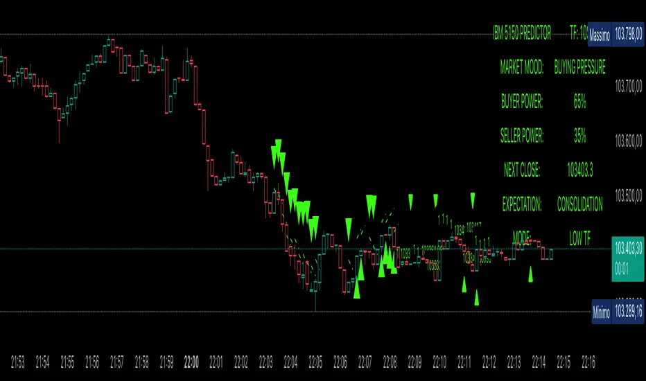
Directional Strength and Momentum Index█ OVERVIEW
“Directional Strength and Momentum Index” (DSMI) is a technical analysis indicator inspired by DMI, but due to different source data, it produces distinct results. DSMI combines direction measurement, trend strength, and overheat levels into a single index, enhanced with gradient fills, extreme zones, entry signals, candle coloring, and a summary table.
█ CONCEPT
The classic DMI, despite its relatively simple logic, can seem somewhat chaotic due to separate +DI and -DI lines and the need for manual interpretation of their relationships. The DSMI indicator was created to increase clarity and speed up results, consolidating key information into a single index from 0 to 100 that simultaneously:
- Indicates trend direction (bullish/bearish)
- Measures movement strength
- Identifies overheat levels
- Generates ready entry signals
DMI (ADX + +DI / -DI) measures trend direction and strength, but does so based solely on comparing price movements between candles. ADX shows whether the trend is orderly and growing (e.g., above 20–30), but does not assess how dynamic the movement is.
DSMI, on the other hand, takes into account candle size and actual market aggression, thus showing directional momentum — whether the trend has real “fuel” to sustain or accelerate, not just whether it is orderly.
The main calculation difference involves replacing True Range with candle size (high-low) and using directional EMA instead of Wilder smoothing. This allows DSMI to react faster to momentum changes, eliminating delays typical of classic DMI based on TR.
This gives the trader an immediate picture of the market situation without analyzing multiple lines.
█ FEATURES
DSMI Main Line:
- EMA(Directional Index) based on +DS and -DS
- Scale 0–100, smooth color gradient depending on strength
+DS / -DS:
- Positive and Negative Directional Strength
- Gradient fill between lines — more intense with stronger trend
Extreme Zones:
- Default 20 and 80
- Gradient fill outside zones
Trend Strength Levels:
- Weak (<10) → neutral
- Moderate (up to 35)
- Strong (up to 45)
- Overheated (up to 55)
- Extreme (>55)
All levels editable
Entry Signals:
- Activated on crossing entry level (default 20)
Or on direction change when DSMI already ≥ entry level
- Highlighted background (green/red)
Candle Coloring:
- According to current trend
Trend Strength Table:
- Top-right corner
- Shows current strength (WEAK/STRONG etc.) + DSMI value
Alerts:
- DSMI Bullish Entry
- DSMI Bearish Entry
█ HOW TO USE
Add to Chart: Paste code in Pine Editor or find in indicator library.
Settings:
DSMI Parameters:
- DSMI Period → default 20
- Show DSMI Line → on/off
Extreme Zones:
- Lower Level → default 20
- Upper Level → default 80
Trend Strength Levels:
- Weak, Moderate, Strong, Overheated → adjust to strategy
Trend Colors:
- BULLISH → default green
- BEARISH → default red
- NEUTRAL → gray
Entry Signals:
- Show Highlight → on/off
- DSMI Entry Level → default 20
Signal Interpretation:
- DSMI Line: Main strength indicator.
- Gradient between +DS and -DS: Visualizes side dominance.
- Crossing 18 with direction confirmation → entry signal.
- Extreme Zones: Potential reversal or continuation points after correction.
- Table: Quick overview of current trend condition.
█ APPLICATIONS
The indicator works well in:
- Trend-following: Enter on signal, exit on direction change or overheat. When a new trend appears, consider entering a position, preferably with a rising trend strength indicator.
- Scalping/daytrading: Shorter period (7–10), lower entry level.
- Swing/position: Longer period (20–30), higher entry level, extreme zones as filters.
- Noise filtering: Ignores consolidation below “Weak” – increasing value e.g. to 15 highlights consolidation zones, but no signals appear there.
Style Adjustment:
- Aggressive strategies → shorten period and entry level
- Conservative → extend period, raise entry level (25–30), watch “Overheated”
“Weak” level (<10 default) → neutral; increasing it e.g. to 15 gives fewer but higher-quality signals. The Weak zone value controls the level below which no signals appear, and the gradient turns gray (often aligned with consolidation zones).
Combine with:
- Support/resistance levels
- Fair Value Gaps (FVG)
- Volume (Volume Profile, VWAP)
- Other oscillators (RSI, Stochastic)
█ NOTES
- Works on all markets and timeframes.
- Adjust period and levels to instrument volatility.
- Higher entry level → fewer signals, higher quality.
- Neutral color below “Weak” – avoids trading in consolidation.
- Gradient and table enable quick assessment without line analysis.

PIVOT-V.13 05-09-25This Pine Script automatically detects pivot levels and generates buy/sell signals based on price action around those pivots. It identifies key support and resistance zones derived from previous period highs, lows, and closes, then marks optimal entry, target, and stop-loss levels on the chart.
The script is designed to assist traders in systematic decision-making using pivot-based strategies.
🔍 Core Features
Automatic Pivot Detection: Calculates and updates pivots in real-time using standard formulas.
Smart Trade Setup:
Buy Signal: Triggered when price action confirms strength above a pivot or resistance level.
Sell Signal: Triggered when price action confirms weakness below a pivot or support level.
Entry, Target & Stop-Loss Levels: Automatically plots potential entry points, stop-loss levels, and take-profit zones based on the nearest pivot structure.
Customizable Settings:
Choose pivot type and timeframe (daily, weekly, or monthly).
Adjust risk ratio, stop size, and confirmation filters.
Enable/disable visual labels or alerts.
Visual Clarity: Clearly marks all pivot levels and trade signals on the chart with colored labels and lines.
🎯 Purpose
This script helps traders quickly identify high-probability entry zones and maintain disciplined trade management by following pre-defined pivot-based rules — reducing emotional bias and enhancing consistency.
Smart Money Flow Index (SMFI) - Advanced SMC [PhenLabs]📊Smart Money Flow Index (SMFI)
Version: PineScript™v6
📌Description
The Smart Money Flow Index (SMFI) is an advanced Smart Money Concepts implementation that tracks institutional trading behavior through multi-dimensional analysis. This comprehensive indicator combines volume-validated Order Block detection, Fair Value Gap identification with auto-mitigation tracking, dynamic Liquidity Zone mapping, and Break of Structure/Change of Character detection into a unified system.
Unlike basic SMC indicators, SMFI employs a proprietary scoring algorithm that weighs five critical factors: Order Block strength (validated by volume), Fair Value Gap size and recency, proximity to Liquidity Zones, market structure alignment (BOS/CHoCH), and multi-timeframe confluence. This produces a Smart Money Score (0-100) where readings above 70 represent optimal institutional setup conditions.
🚀Points of Innovation
Volume-Validated Order Block Detection – Only displays Order Blocks when formation candle exceeds customizable volume multiplier (default 1.5x average), filtering weak zones and highlighting true institutional accumulation/distribution
Auto-Mitigation Tracking System – Fair Value Gaps and Order Blocks automatically update status when price mitigates them, with visual distinction between active and filled zones preventing trades on dead levels
Proprietary Smart Money Score Algorithm – Combines weighted factors (OB strength 25%, FVG proximity 20%, Liquidity 20%, Structure 20%, MTF 15%) into single 0-100 confidence rating updating in real-time
ATR-Based Adaptive Calculations – All distance measurements use 14-period Average True Range ensuring consistent function across any instrument, timeframe, or volatility regime without manual recalibration
Dynamic Age Filtering – Automatically removes liquidity levels and FVGs older than configurable thresholds preventing chart clutter while maintaining relevant levels
Multi-Timeframe Confluence Integration – Analyzes higher timeframe bias with customizable multipliers (2-10x) and incorporates HTF trend direction into Smart Money Score for institutional alignment
🔧Core Components
Order Block Engine – Detects institutional supply/demand zones using characteristic patterns (down-move-then-strong-up for bullish, up-move-then-strong-down for bearish) with minimum volume threshold validation, tracks mitigation when price closes through zones
Fair Value Gap Scanner – Identifies price imbalances where current candle's low/high leaves gap with two-candle-prior high/low, filters by minimum size percentage, monitors 50% fill for mitigation status
Liquidity Zone Mapper – Uses pivot high/low detection with configurable lookback to mark swing points where stop losses cluster, extends horizontal lines to visualize sweep targets, manages lifecycle through age-based removal
Market Structure Analyzer – Tracks pivot progression to identify trend through higher-highs/higher-lows (bullish) or lower-highs/lower-lows (bearish), detects Break of Structure and Change of Character for trend/reversal confirmation
Scoring Calculation Engine – Evaluates proximity to nearest Order Blocks using ATR-normalized distance, assesses FVG recency and distance, calculates liquidity proximity with age weighting, combines structure bias and MTF trend into smoothed final score
🔥Key Features
Customizable Display Limits – Control maximum Order Blocks (1-10), Liquidity Zones (1-10), and FVG age (10-200 bars) to maintain clean charts focused on most relevant institutional levels
Gradient Strength Visualization – All zones render with transparency-adjustable coloring where stronger/newer zones appear more solid and weaker/older zones fade progressively providing instant visual hierarchy
Educational Label System – Optional labels identify each zone type (Bullish OB, Bearish OB, Bullish FVG, Bearish FVG, BOS) with color-coded text helping traders learn SMC concepts through practical application
Real-Time Smart Money Score Dashboard – Top-right table displays current score (0-100) with color coding (green >70, yellow 30-70, red <30) plus trend arrow for at-a-glance confidence assessment
Comprehensive Alert Suite – Configurable notifications for Order Block formation, Fair Value Gap detection, Break of Structure events, Change of Character signals, and high Smart Money Score readings (>70)
Buy/Sell Signal Integration – Automatically plots triangle markers when Smart Money Score exceeds 70 with aligned market structure and fresh Order Block detection providing clear entry signals
🎨Visualization
Order Block Boxes – Shaded rectangles extend from formation bar spanning high-to-low of institutional candle, bullish zones in green, bearish in red, with customizable transparency (80-98%)
Fair Value Gap Zones – Rectangular areas marking imbalances, active FVGs display in bright colors with adjustable transparency, mitigated FVGs switch to gray preventing trades on filled zones
Liquidity Level Lines – Dashed horizontal lines extend from pivot creation points, swing highs in bearish color (short targets above), swing lows in bullish color (long targets below), opacity decreases with age
Structure Labels – "BOS" labels appear above/below price when Break of Structure confirmed, colored by direction (green bullish, red bearish), positioned at 1% beyond highs/lows for visibility
Educational Info Panel – Bottom-right table explains key terminology (OB, FVG, BOS, CHoCH) and score interpretation (>70 high probability) with semi-transparent background for readability
📖Usage Guidelines
General Settings
Show Order Blocks – Default: On, toggles visibility of institutional supply/demand zones, disable when focusing solely on FVGs or Liquidity
Show Fair Value Gaps – Default: On, controls FVG zone display including active and mitigated imbalances
Show Liquidity Zones – Default: On, manages liquidity line visibility, disable on lower timeframes to reduce clutter
Show Market Structure – Default: On, toggles BOS/CHoCH label display
Show Smart Money Score – Default: On, controls score dashboard visibility
Order Block Settings
OB Lookback Period – Default: 20, Range: 5-100, controls bars scanned for Order Block patterns, lower values detect recent activity, higher values find older blocks
Min Volume Multiplier – Default: 1.5, Range: 1.0-5.0, sets minimum volume threshold as multiple of 20-period average, higher values (2.0+) filter for strongest institutional candles
Max Order Blocks to Display – Default: 3, Range: 1-10, limits simultaneous Order Blocks shown, lower settings (1-3) maintain focus on most recent zones
Fair Value Gap Settings
Min FVG Size (%) – Default: 0.3, Range: 0.1-2.0, defines minimum gap size as percentage of close price, lower values detect micro-imbalances, higher values focus on significant gaps
Max FVG Age (bars) – Default: 50, Range: 10-200, removes FVGs older than specified bars, lower settings (10-30) for scalping, higher (100-200) for swing trading
Show FVG Mitigation – Default: On, displays filled FVGs in gray providing visual history, disable to show only active untouched imbalances
Liquidity Zone Settings
Liquidity Lookback – Default: 50, Range: 20-200, sets pivot detection period for swing highs/lows, lower values (20-50) mark shorter-term liquidity, higher (100-200) identify major swings
Max Liquidity Age (bars) – Default: 100, Range: 20-500, removes liquidity lines older than specified bars, adjust based on timeframe
Liquidity Sensitivity – Default: 0.5, Range: 0.1-1.0, controls pivot detection sensitivity, lower values mark only major swings, higher values identify minor swings
Max Liquidity Zones to Display – Default: 3, Range: 1-10, limits total liquidity levels shown maintaining chart clarity
Market Structure Settings
Pivot Length – Default: 5, Range: 3-15, defines bars to left/right for pivot validation, lower values (3-5) create sensitive structure breaks, higher (10-15) filter for major shifts
Min Structure Move (%) – Default: 1.0, Range: 0.1-5.0, sets minimum percentage move required between pivots to confirm structure change
Multi-Timeframe Settings
Enable MTF Analysis – Default: On, activates higher timeframe trend analysis incorporation into Smart Money Score
Higher Timeframe Multiplier – Default: 4, Range: 2-10, multiplies current timeframe to determine analysis timeframe (4x on 15min = 1hour)
Visual Settings
Bullish Color – Default: Green (#089981), sets color for bullish Order Blocks, FVGs, and structure elements
Bearish Color – Default: Red (#f23645), defines color for bearish elements
Neutral Color – Default: Gray (#787b86), controls color of mitigated zones and neutral elements
Show Educational Labels – Default: On, displays text labels on zones identifying type (OB, FVG, BOS), disable once familiar with patterns
Order Block Transparency – Default: 92, Range: 80-98, controls Order Block box transparency
FVG Transparency – Default: 92, Range: 80-98, sets Fair Value Gap zone transparency independently from Order Blocks
Alert Settings
Alert on Order Block Formation – Default: On, triggers notification when new volume-validated Order Block detected
Alert on FVG Formation – Default: On, sends alert when Fair Value Gap appears enabling quick response to imbalances
Alert on Break of Structure – Default: On, notifies when BOS or CHoCH confirmed
Alert on High Smart Money Score – Default: On, alerts when Smart Money Score crosses above 70 threshold indicating high-probability setup
✅Best Use Cases
Order Block Retest Entries – After Break of Structure, wait for price retrace into fresh bullish Order Block with Smart Money Score >70, enter long on zone reaction targeting next liquidity level
Fair Value Gap Retracement Trading – When price creates FVG during strong move then retraces, enter as price approaches unfilled gap expecting institutional orders to continue trend
Liquidity Sweep Reversals – Monitor price approaching swing high/low liquidity zones against prevailing Smart Money Score trend, after stop hunt sweep watch for rejection into premium Order Block/FVG
Multi-Timeframe Confluence Setups – Identify alignment when current timeframe Order Block coincides with higher timeframe FVG plus MTF analysis showing matching trend bias
Break of Structure Continuations – After BOS confirms trend direction, trade pullbacks to nearest Order Block or FVG in direction of structure break using Smart Money Score >70 as entry filter
Change of Character Reversal Plays – When CHoCH detected indicating potential reversal, look for Smart Money Score pivot with opposing Order Block formation then enter on structure confirmation
⚠️Limitations
Lagging Pivot Calculations – Pivot-based features (Liquidity Zones, Market Structure) require bars to right of pivot for confirmation, meaning these elements identify levels retrospectively with delay equal to lookback period
Whipsaw in Ranging Markets – During choppy conditions, Order Blocks fail frequently and structure breaks produce false signals as Smart Money Score fluctuates without clear institutional bias, best used in trending markets
Volume Data Dependency – Order Block volume validation requires accurate volume data which may be incomplete on Forex pairs or limited in crypto exchange feeds
Subjectivity in Scoring Weights – Proprietary 25-20-20-20-15 weighting reflects general institutional behavior but may not optimize for specific instruments or market regimes, user cannot adjust factor weights
Visual Complexity on Lower Timeframes – Sub-hour timeframes generate excessive zones creating cluttered charts, requires aggressive display limit reduction and higher minimum thresholds
No Fundamental Integration – Indicator analyzes purely technical price action and volume without incorporating economic events, news catalysts, or fundamental shifts that override technical levels
💡What Makes This Unique
Unified SMC Ecosystem – Unlike indicators displaying Order Blocks OR FVGs OR Liquidity separately, SMFI combines all three institutional concepts plus market structure into single cohesive system
Proprietary Confidence Scoring – Rather than manual setup assessment, automated Smart Money Score quantifies probability by weighting five institutional dimensions into actionable 0-100 rating
Volume-Filtered Quality – Eliminates weak Order Blocks forming without institutional volume confirmation, ensuring displayed zones represent genuine accumulation/distribution
Adaptive Lifecycle Management – Automatically updates mitigation status and removes aged zones preventing trades on dead levels through continuous validity and age monitoring
Educational Integration – Built-in tooltips, labeled zones, and reference panel make indicator functional for both learning Smart Money Concepts and executing strategies
🔬How It Works
Order Block Detection – Scans for patterns where strong directional move follows counter-move creating last down-candle before rally (bullish OB) or last up-candle before sell-off (bearish OB), validates formations only when candle exhibits volume exceeding configurable multiple (default 1.5x) of 20-bar average volume
Fair Value Gap Identification – Compares current candle’s high/low against two-candles-prior low/high to detect price imbalances, calculates gap size as percentage of close and filters micro-gaps below minimum threshold (default 0.3%), monitors whether subsequent price fills 50% triggering mitigation status
Liquidity Zone Mapping – Employs pivot detection using configurable lookback (default 50 bars) to identify swing highs/lows where retail stops cluster, extends horizontal reference lines from pivot creation and applies age-based filtering to remove stale zones
Market Structure Analysis – Tracks pivot progression using structure-specific lookback (default 5 bars) to determine trend, confirms uptrend when new pivot high exceeds previous by minimum move percentage, detects Break of Structure when price breaks recent pivot level, flags Change of Character for potential reversals
Multi-Timeframe Confluence – When enabled, requests security data from higher timeframe (current TF × HTF multiplier, default 4x), compares HTF close against HTF 20-period MA to determine bias, contributes ±50 points to score ensuring alignment with institutional positioning on superior timeframe
Smart Money Score Calculation – Evaluates Order Block component via ATR-normalized distance producing max 100-point contribution weighted at 25%, assesses FVG factor through age penalty and distance at 20% weight, calculates Liquidity proximity at 20%, incorporates structure bias (±50-100 points) at 20%, adds MTF component at 15%, applies 3-period smoothing to reduce volatility
Visual Rendering and Lifecycle – Draws Order Block boxes, Fair Value Gap rectangles with color coding (green/red active, gray mitigated), extends liquidity dashed lines with fade-by-age opacity, plots BOS labels, displays Smart Money Score dashboard, continuously updates checking mitigation conditions and removing elements exceeding age/display limits
💡Note:
The Smart Money Flow Index combines multiple Smart Money Concepts into unified institutional order flow analysis. For optimal results, use the Smart Money Score as confluence filter rather than standalone entry signal – scores above 70 indicate high-probability setups but should be combined with risk management, higher timeframe bias, and market regime understanding.
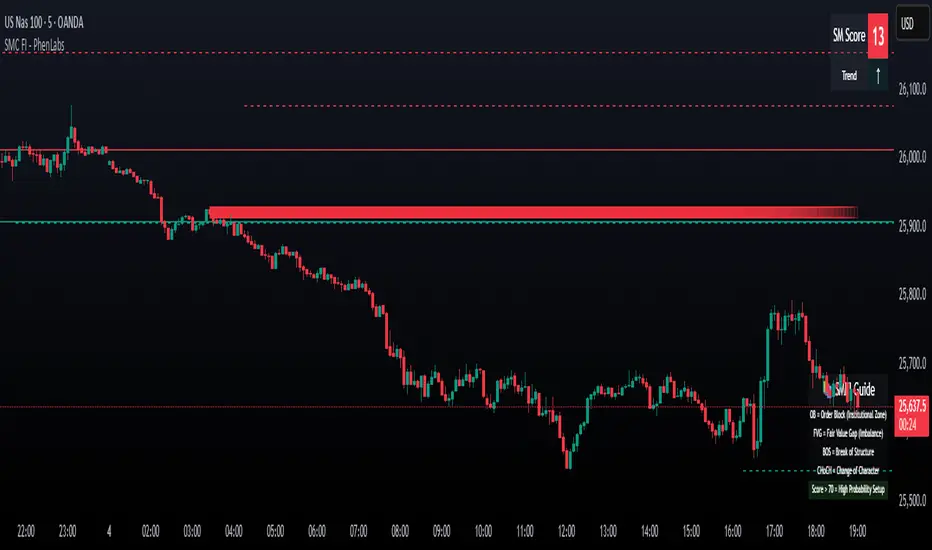
Volume Area 80 Rule Pro - Adaptive RTHSummary in one paragraph
Adaptive value area 80 percent rule for index futures large cap equities liquid crypto and major FX on intraday timeframes. It focuses activity only when multiple context gates align. It is original because the classic prior day value area traverse is fused with a daily regime classifier that remaps the operating parameters in real time.
Scope and intent
• Markets. ES NQ SPY QQQ large cap equities BTC ETH major FX pairs and other liquid RTH instruments
• Timeframes. One minute to one hour with daily regime context
• Default demo used in the publication. ES1 on five minutes
• Purpose. Trade only the balanced days where the 80 percent traverse has edge while standing aside or tightening rules during trend or shock
Originality and usefulness
• Unique fusion. Prior day value area logic plus a rolling daily regime classifier using percentile ranks of realized volatility and ADX. The regime remaps hold time end of window stop buffer and value area coverage on each session
• Failure mode addressed. False starts during strong trend or shock sessions and weak traverses during quiet grind
• Testability. All gates are visible in Inputs and debug flags can be plotted so users can verify why a suggestion appears
• Portable yardstick. The regime uses ATR divided by close and ADX percent ranks which behave consistently across symbols
Method overview in plain language
The script builds the prior session profile during regular trading hours. At the first regular bar it freezes yesterday value area low value area high and point of control. It then evaluates the current session open location the first thirty minute volume rank the open gap rank and an opening drive test. In parallel a daily series classifies context into Calm Balance Trend or Shock from rolling percentile ranks of realized volatility and ADX. The classifier scales the rules. Calm uses longer holds and a slightly wider value area. Trend and Shock shorten the window reduce holds and enlarge stop buffers.
Base measures
• Range basis. True Range smoothed over a configurable length on both the daily and intraday series
• Return basis. Not required. ATR over close is the unit for regime strength
Components
• Prior Value Area Engine. Builds yesterday value area low value area high and point of control from a binned volume profile with automatic TPO fallback and minimum integrity guards
• Opening Location. Detects whether the session opens above the prior value area or below it
• Inside Hold Counter. Counts consecutive bars that hold inside the value area after a re entry
• Volume Gate. Percentile of the first thirty minutes volume over a rolling sample
• Gap Gate. Percentile rank of the regular session open gap over a rolling sample
• Drive Gate. Opening drive check using a multiple of intraday ATR
• Regime Classifier. Percentile ranks of daily ATR over close and daily ADX classify Calm Balance Trend Shock and remap parameters
• Session windows optional. Windows follow the chart exchange time
Fusion rule
Minimum satisfied gates approach. A re entry must hold inside the value area for a regime scaled number of bars while the volume gap and drive gates allow the setup. The regime simultaneously scales value area coverage end minute time stop and stop buffer.
Signal rule
• Long suggestion appears when price opens below yesterday value area then re enters and holds for the required bars while all gates allow the setup
• Short suggestion appears when price opens above yesterday value area then re enters and holds for the required bars while all gates allow the setup
• WAIT shows implicitly when any required gate is missing
• Exit labels mark target touch stop touch or a time based close
Inputs with guidance
Setup
• Signal timeframe. Uses the chart by default
• Session windows optional. Start and end minutes inside regular trading hours
• Invert direction is not used. The logic is symmetric
Logic
• Hold bars inside value area. Typical range 3 to 12. Raising it reduces trades and favors better traverses. Lowering it increases frequency and risk of false starts
• Earliest minute since RTH open and Latest minute since RTH open. Typical range 0 to 390. Reducing the latest minute cuts late session trades
• Time stop bars after entry. Typical range 6 to 30. Larger values give setups more room
Filters
• Value area coverage. Typical range 0.70 to 0.85. Higher coverage narrows the traverse but accepts fewer days
• Bin size in ticks. Typical range 1 to 8. Larger bins stabilize noisy profiles
• Stop buffer ticks beyond edge. Typical range 2 to 20. Larger buffers survive noise
• First thirty minute volume percentile. Typical range 0.30 to 0.70. Higher values require more active opens
• Gap filter percentile. Typical range 0.70 to 0.95. Lower values block more gap days
• Opening drive multiple and bars. Higher multiple or longer bars block strong directional opens
Adaptivity
• Lookback days for regime ranks. Typical 150 to 500
• Calm RV percentile. Typical 25 to 45
• Trend ADX percentile. Typical 55 to 75
• Shock RV percentile. Typical 75 to 90
• End minute ratio in Trend and Shock. Typical 0.5 to 0.8
• Hold and Time stop scales per regime. Use values near one to keep behavior close to static settings
Realism and responsible publication
• No performance claims. Past results never guarantee future outcomes
• Shapes can move while a bar forms and settle on close
• Sessions use the chart exchange time
Honest limitations and failure modes
• Economic releases and thin liquidity can break the balance premise
• Gap heavy symbols may work better with stronger gap filters and a True Range focus
• Very quiet regimes reduce signal contrast. Consider longer windows or higher thresholds
Legal
Education and research only. Not investment advice. Test in simulation before any live use.

MTC – Multi-Timeframe Trend ConfirmatorMTC – Multi-Timeframe Trend Confirmator
The Ultimate Multi-Timeframe Trend Analysis Tool
MTC v6 is a comprehensive trend confirmation indicator that analyzes market conditions across multiple timeframes simultaneously. It combines six powerful technical indicators to give you a clear, visual representation of trend strength and direction.
🎯 Key Features
Visual Trend Gauge
Real-time trend strength display for 3 customizable timeframes
Progressive bar visualization (fills from left to right)
Color-coded signals: 🟢 Green (Bullish) | 🔴 Red (Bearish) | 🟡 Yellow (Ranging)
Score range: -10 to +10 for precise trend measurement
Multi-Indicator Analysis
The indicator combines 6 proven technical tools:
EMA 200 – Long-term trend direction
SMA 50/200 – Golden/Death cross signals
RSI 14 – Momentum confirmation
MACD – Trend strength validation
ADX (>25) – Trend intensity measurement (2x weight)
Supertrend – Dynamic support/resistance (2x weight)
⚙️ Customization Options
Flexible Timeframes: Set any timeframes you prefer (default: 15M, 1H, 4H)
Adjustable Gauge Size: Small, Medium, or Large display
Toggle Indicators: Enable/disable any of the 6 technical indicators
Supertrend Settings: Customize factor and ATR period
Built-in Alerts: Get notified when trends confirm
📈 How to Use
Score Interpretation:
Score > +2 = Bullish trend
Score < -2 = Bearish trend
Score between -2 and +2 = Ranging/Neutral
Multi-Timeframe Confirmation:
Look for alignment across timeframes for strongest signals
Higher timeframes confirm the overall trend direction
Lower timeframes help with precise entry timing
Visual Background:
Green background = Confirmed uptrend (Higher + Mid TF aligned)
Red background = Confirmed downtrend (Higher + Mid TF aligned)
💡 Perfect For
Swing traders seeking trend confirmation
Day traders analyzing multiple timeframes
Position traders validating long-term trends
Anyone who wants clear, visual trend analysis
Trade with confidence. Trade with confirmation. Trade with MTC
-Natantia

NY ORB - Full Dynamic SystemNY ORB - Full Dynamic Strategy Summary
1. Opening Range and Session Timing
Opening Range (ORB) Calculation: The strategy identifies the ORB High and ORB Low by tracking the highest high and lowest low during the specified New York pre-market window, which is set by default from 8:30 to 8:45 (New York time).
Entry Window: Trading activity is restricted to a specific entry period, typically starting shortly after the ORB is established (default: 8:50 to 12:00).
Hard Exit Time: Any remaining open positions are automatically closed at a fixed exit time (default: 13:25).
2. Trade Entry Logic and Filters
An entry (Long or Short) is generated when the price breaks out of the established ORB, provided it passes a series of optional filters:
Direction Control: The user can restrict the strategy to trade Long Only, Short Only, or Both.
Second Breakout Logic: An optional filter that requires the price to break out, reverse back into the range, and then break out again, confirming momentum after a consolidation.
Confirmation Candle Count: An optional filter that checks the close of a previous candle (e.g., 1 or 2 candles ago) to ensure the price was still inside the range, preventing premature entry.
Technical Filters (Optional): The entry is only executed if it aligns with selected indicators:
RSI: Filters for non-overbought (Long) or non-oversold (Short) conditions.
MACD: Requires the MACD line to be above/below the Signal line for alignment.
VWAP: Requires the price to be above/below the Volume-Weighted Average Price.
Trend Filter (SMMA): Requires the price to be above/below a 50-period Simple Moving Average.
3. Dynamic Risk and Exit Management
This strategy features highly configurable stop-loss and profit-taking mechanics:
Primary Stop Loss Methods: The Stop Loss distance can be dynamically chosen from four types:
Fixed: A fixed number of ticks.
ATR: Based on a multiple of the Average True Range (ATR).
Capped ATR: ATR-based, but with a hard maximum tick limit.
OR-Based: Based on a multiple of the actual ORB High-to-Low range.
Dynamic Profit Target: The Take Profit level is calculated dynamically based on a multiplier of either the ATR or the ORB Range.
Breakeven Stop:
If enabled, the Stop Loss automatically moves to the entry price (Breakeven) once the price moves a predetermined distance in the profitable direction.
An Adaptive Breakeven option allows the trigger distance to be calculated as a percentage of the overall ATR Profit Target.
Trailing Stop: The strategy uses a trailing stop, which can be custom-set (fixed ticks) or dynamically tied to the ATR. An optional feature Auto Tighten Trailing reduces the trailing multiplier once the breakeven level is hit.
MA Cross Exit: An alternative, counter-trend exit mechanism that closes the trade if the price crosses back over the chosen Moving Average (either SMMA or VWAP), overriding the pending profit target.
4. Daily Account Management
The strategy includes crucial daily risk controls to protect capital and lock in profits:
Daily Profit Limit: If the total daily PnL (realized and unrealized) hits a predefined maximum profit threshold (in ticks), all trades are closed, and new entries are blocked for the remainder of the trading day.
Daily Loss Limit: Conversely, if the total daily PnL hits a predefined maximum loss threshold, all trades are closed, and new entries are blocked for the remainder of the day.

RSI Trendline Pro - Multi Confirmation
Overview
RSI Trendline Pro is an advanced Pine Script indicator that automatically draws trendlines on the RSI (Relative Strength Index) to detect support and resistance breakouts. It generates high-quality trading signals through a multi-confirmation system.
Key Features
Auto Trendlines: Detects pivot points on RSI to create intelligent support and resistance lines
Multi-Confirmation System: Combines Volume, Stochastic RSI, ADX, and Divergence filters to reduce false signals
RSI Divergence Detection: Automatically identifies bullish/bearish divergences between price and RSI
Live Dashboard: Displays RSI value, active trendlines, ADX strength, and last signal info on a visual panel
Smart Breakout Detection: Identifies trendline breaks and generates LONG/SHORT signals
How to Use
Add to TradingView: Paste code into Pine Editor and add to chart
Configure Parameters:
RSI Length: RSI period (default: 14)
Pivot Strength: Trendline sensitivity (lower = more lines)
Filters: Enable/disable Volume, Divergence, Stoch RSI, and ADX confirmations
Follow Signals:
LONG (Green): When RSI breaks resistance upward
SHORT (Red): When RSI breaks support downward
Divergence: "D" markers indicate potential trend reversals
Alert Setup
Script offers 4 alert types:
LONG Breakout: Resistance break
SHORT Breakout: Support break
Bullish/Bearish Divergence: Divergence detection
Any Signal: Combined alert for all signals
Best Practices
Prioritize high-volume breakouts (Volume Filter enabled)
Trends are stronger when ADX > 25
Confirm divergence signals with price action
Trade when 2-3 confirmations align

Opening Range Breakout with Multi-Timeframe Liquidity]═══════════════════════════════════════
OPENING RANGE BREAKOUT WITH MULTI-TIMEFRAME LIQUIDITY
═══════════════════════════════════════
A professional Opening Range Breakout (ORB) indicator enhanced with multi-timeframe liquidity detection, trading session visualization, volume analysis, and trend confirmation tools. Designed for intraday trading with comprehensive alert system.
───────────────────────────────────────
WHAT THIS INDICATOR DOES
───────────────────────────────────────
This indicator combines multiple trading concepts:
- Opening Range Breakout (ORB) - Customizable time period detection with automatic high/low identification
- Multi-Timeframe Liquidity - HTF (Higher Timeframe) and LTF (Lower Timeframe) key level detection
- Trading Sessions - Tokyo, London, New York, and Sydney session visualization
- Volume Analysis - Volume spike detection and strength measurement
- Multi-Timeframe Confirmation - Trend bias from higher timeframes
- EMA Integration - Trend filter and dynamic support/resistance
- Smart Alerts - Quality-filtered breakout notifications
───────────────────────────────────────
HOW IT WORKS
───────────────────────────────────────
OPENING RANGE BREAKOUT (ORB):
Concept:
The Opening Range is a period at the start of a trading session where price establishes an initial high and low. Breakouts beyond this range often indicate the direction of the day's trend.
Detection Method:
- Default: 15-minute opening range (configurable)
- Custom Range: Set specific session times with timezone support
- Automatically identifies ORH (Opening Range High) and ORL (Opening Range Low)
- Tracks ORB mid-point for reference
Range Establishment:
1. Session starts (or custom time begins)
2. Tracks highest high and lowest low during the period
3. Range confirmed at end of opening period
4. Levels extend throughout the session
Breakout Detection:
- Bullish Breakout: Close above ORH
- Bearish Breakout: Close below ORL
- Mid-point acts as bias indicator
Visual Display:
- Shaded box during range formation
- Horizontal lines for ORH, ORL, and mid-point
- Labels showing level values
- Color-coded fills based on selected method
Fill Color Methods:
1. Session Comparison:
- Green: Current OR mid > Previous OR mid
- Red: Current OR mid < Previous OR mid
- Gray: Equal or first session
- Shows day-over-day momentum
2. Breakout Direction (Recommended):
- Green: Price currently above ORH (bullish breakout)
- Red: Price currently below ORL (bearish breakout)
- Gray: Price inside range (no breakout)
- Real-time breakout status
MULTI-TIMEFRAME LIQUIDITY:
Two-Tier System for comprehensive level identification:
HTF (Higher Timeframe) Key Liquidity:
- Default: 4H timeframe (configurable to Daily, Weekly)
- Identifies major institutional levels
- Uses pivot detection with adjustable parameters
- Suitable for swing highs/lows where large orders rest
LTF (Lower Timeframe) Key Liquidity:
- Default: 1H timeframe (configurable)
- Provides precision entry/exit levels
- Finer granularity for intraday trading
- Captures minor swing points
Calculation Method:
- Pivot high/low detection algorithm
- Configurable left bars (lookback) and right bars (confirmation)
- Timeframe multiplier for accurate multi-timeframe detection
- Automatic level extension
Mitigation System:
- Tracks when levels are swept (broken)
- Configurable mitigation type: Wick or Close-based
- Option to remove or show mitigated levels
- Display limit prevents chart clutter
Asset-Specific Optimization:
The indicator includes quick reference settings for different assets:
- Major Forex (EUR/USD, GBP/USD): Default settings optimal
- Crypto (BTC/ETH): Left=12, Right=4, Display=7
- Gold: HTF=1D, Left=20
TRADING SESSIONS:
Four Major Sessions with Full Customization:
Tokyo Session:
- Default: 04:00-13:00 UTC+4
- Asian trading hours
- Often sets daily range
London Session:
- Default: 11:00-20:00 UTC+4
- Highest liquidity period
- Major institutional activity
New York Session:
- Default: 16:00-01:00 UTC+4
- US market hours
- High-impact news events
Sydney Session:
- Default: 01:00-10:00 UTC+4
- Earliest Asian activity
- Lower volatility
Session Features:
- Shaded background boxes
- Session name labels
- Optional open/close lines
- Session high/low tracking with colored lines
- Each session has independent color settings
- Fully customizable times and timezones
VOLUME ANALYSIS:
Volume-Based Trade Confirmation:
Volume MA:
- Configurable period (default: 20)
- Establishes average volume baseline
- Used for spike detection
Volume Spike Detection:
- Identifies when volume exceeds MA * multiplier
- Default: 1.5x average volume
- Confirms breakout strength
Volume Strength Measurement:
- Calculates current volume as percentage of average
- Shows relative volume intensity
- Used in alert quality filtering
High Volume Bars:
- Identifies bars above 50th percentile
- Additional confirmation layer
- Indicates institutional participation
MULTI-TIMEFRAME CONFIRMATION:
Trend Bias from Higher Timeframes:
HTF 1 (Trend):
- Default: 1H timeframe
- Uses EMA to determine intermediate trend
- Compares current timeframe EMA to HTF EMA
HTF 2 (Bias):
- Default: 4H timeframe
- Uses 50 EMA for longer-term bias
- Confirms overall market direction
Bias Classifications:
- Bullish Bias: HTF close > HTF 50 EMA AND Current EMA > HTF1 EMA
- Bearish Bias: HTF close < HTF 50 EMA AND Current EMA < HTF1 EMA
- Neutral Bias: Mixed signals between timeframes
EMA Stack Analysis:
- Compares EMA alignment across timeframes
- +1: Bullish stack (lower TF EMA > higher TF EMA)
- -1: Bearish stack (lower TF EMA < higher TF EMA)
- 0: Neutral/crossed
Usage:
- Filters false breakouts
- Confirms trend direction
- Improves trade quality
EMA INTEGRATION:
Dynamic EMA for Trend Reference:
Features:
- Configurable period (default: 20)
- Customizable color and width
- Acts as dynamic support/resistance
- Trend filter for ORB trades
Application:
- Above EMA: Favor long breakouts
- Below EMA: Favor short breakouts
- EMA cross: Potential trend change
- Distance from EMA: Momentum gauge
SMART ALERT SYSTEM:
Quality-Filtered Breakout Notifications:
Alert Types:
1. Standard ORB Breakout
2. High Quality ORB Breakout
Quality Criteria:
- Volume Confirmation: Volume > 1.2x average
- MTF Confirmation: Bias aligned with breakout direction
Standard Alert:
- Basic breakout detection
- Price crosses ORH or ORL
- Icon: 🚀 (bullish) or 🔻 (bearish)
High Quality Alert:
- Both volume AND MTF confirmed
- Stronger probability setup
- Icon: 🚀⭐ (bullish) or 🔻⭐ (bearish)
Alert Information Includes:
- Alert quality rating
- Breakout level and current price
- Volume strength percentage (if enabled)
- MTF bias status (if enabled)
- Recommended action
One Alert Per Bar:
- Prevents alert spam
- Uses flag system to track sent alerts
- Resets on new ORB session
───────────────────────────────────────
HOW TO USE
───────────────────────────────────────
OPENING RANGE SETUP:
Basic Configuration:
1. Select time period for opening range (default: 15 minutes)
2. Choose fill color method (Breakout Direction recommended)
3. Enable historical data display if needed
Custom Range (Advanced):
1. Enable Custom Range toggle
2. Set specific session time (e.g., 0930-0945)
3. Select appropriate timezone
4. Useful for specific market opens (NYSE, LSE, etc.)
LIQUIDITY LEVELS SETUP:
Quick Configuration by Asset:
- Forex: Use default settings (Left=15, Right=5)
- Crypto: Set Left=12, Right=4, Display=7
- Gold: Set HTF=1D, Left=20
HTF Liquidity:
- Purpose: Major support/resistance levels
- Recommended: 4H for day trading, 1D for swing trading
- Use as profit targets or reversal zones
LTF Liquidity:
- Purpose: Entry/exit refinement
- Recommended: 1H for day trading, 4H for swing trading
- Use for position management
Mitigation Settings:
- Wick-based: More sensitive (default)
- Close-based: More conservative
- Remove or Show mitigated levels based on preference
TRADING SESSIONS SETUP:
Enable/Disable Sessions:
- Master toggle for all sessions
- Individual session controls
- Show/hide session names
Session High/Low Lines:
- Enable to see session extremes
- Each session has custom colors
- Useful for range trading
Customization:
- Adjust session times for your broker
- Set timezone to match your location
- Customize colors for visibility
VOLUME ANALYSIS SETUP:
Enable Volume Analysis:
1. Toggle on Volume Analysis
2. Set MA length (20 recommended)
3. Adjust spike multiplier (1.5 typical)
Usage:
- Confirm breakouts with volume
- Identify climactic moves
- Filter false signals
MULTI-TIMEFRAME SETUP:
HTF Selection:
- HTF 1 (Trend): 1H for day trading, 4H for swing
- HTF 2 (Bias): 4H for day trading, 1D for swing
Interpretation:
- Trade only with bias alignment
- Neutral bias: Be cautious
- Bias changes: Potential reversals
EMA SETUP:
Configuration:
- Period: 20 for responsive, 50 for smoother
- Color: Choose contrasting color
- Width: 1-2 for visibility
Usage:
- Filter trades: Long above, Short below
- Dynamic support/resistance reference
- Trend confirmation
ALERT SETUP:
TradingView Alert Creation:
1. Enable alerts in indicator settings
2. Enable ORB Breakout Alerts
3. Right-click chart → Add Alert
4. Select this indicator
5. Choose "Any alert() function call"
6. Configure delivery method (mobile, email, webhook)
Alert Filtering:
- All alerts include quality rating
- High Quality alerts = Volume + MTF confirmed
- Standard alerts = Basic breakout only
───────────────────────────────────────
TRADING STRATEGIES
───────────────────────────────────────
CLASSIC ORB STRATEGY:
Setup:
1. Wait for opening range to complete
2. Price breaks and closes above ORH or below ORL
3. Volume > average (if enabled)
4. MTF bias aligned (if enabled)
Entry:
- Bullish: Buy on break above ORH
- Bearish: Sell on break below ORL
- Consider retest entries for better risk/reward
Stop Loss:
- Bullish: Below ORL or range mid-point
- Bearish: Above ORH or range mid-point
- Adjust based on volatility
Targets:
- Initial: Range width extension (ORH + range width)
- Secondary: HTF liquidity levels
- Final: Session high/low or major support/resistance
ORB + LIQUIDITY CONFLUENCE:
Enhanced Setup:
1. Opening range established
2. HTF liquidity level near or beyond ORH/ORL
3. Breakout occurs with volume
4. Price targets the liquidity level
Entry:
- Enter on ORB breakout
- Target the HTF liquidity level
- Use LTF liquidity for position management
Management:
- Partial profits at ORB + range width
- Move stop to breakeven at LTF liquidity
- Final exit at HTF liquidity sweep
ORB REJECTION STRATEGY (Counter-Trend):
Setup:
1. Price breaks above ORH or below ORL
2. Weak volume (below average)
3. MTF bias opposite to breakout
4. Price closes back inside range
Entry:
- Failed bullish break: Short below ORH
- Failed bearish break: Long above ORL
Stop Loss:
- Beyond the failed breakout level
- Or beyond session extreme
Target:
- Opposite end of opening range
- Range mid-point for partial profit
SESSION-BASED ORB TRADING:
Tokyo Session:
- Typically narrower ranges
- Good for range trading
- Wait for London open breakout
London Session:
- Highest volume and volatility
- Strong ORB setups
- Major liquidity sweeps common
New York Session:
- Strong trending moves
- News-driven volatility
- Good for momentum trades
Sydney Session:
- Quieter conditions
- Suitable for range strategies
- Sets up Tokyo session
EMA-FILTERED ORB:
Rules:
- Only take bullish breaks if price > EMA
- Only take bearish breaks if price < EMA
- Ignore counter-trend breaks
Benefits:
- Reduces false signals
- Aligns with larger trend
- Improves win rate
───────────────────────────────────────
CONFIGURATION GUIDE
───────────────────────────────────────
OPENING RANGE SETTINGS:
Time Period:
- 15 min: Standard for most markets
- 30 min: Wider range, fewer breakouts
- 60 min: For slower markets or swing trades
Custom Range:
- Use for specific market opens
- NYSE: 0930-1000 EST
- LSE: 0800-0830 GMT
- Set timezone to match exchange
Historical Display:
- Enable: See all previous session data
- Disable: Cleaner chart, current session only
LIQUIDITY SETTINGS:
Left Bars (5-30):
- Lower: More frequent, sensitive levels
- Higher: Fewer, more significant levels
- Recommended: 15 for most markets
Right Bars (1-25):
- Confirmation period
- Higher: More reliable, less frequent
- Recommended: 5 for balance
Display Limit (1-20):
- Number of active levels shown
- Higher: More context, busier chart
- Recommended: 7 for clarity
Extension Options:
- Short: Levels visible near formation
- Current: Extended to current bar (recommended)
- Max: Extended indefinitely
VOLUME SETTINGS:
MA Length (5-50):
- Shorter: More responsive to spikes
- Longer: Smoother baseline
- Recommended: 20 for balance
Spike Multiplier (1.0-3.0):
- Lower: More sensitive spike detection
- Higher: Only extreme spikes
- Recommended: 1.5 for day trading
MULTI-TIMEFRAME SETTINGS:
HTF 1 (Trend):
- 5m chart: Use 15m or 1H
- 15m chart: Use 1H or 4H
- 1H chart: Use 4H or 1D
HTF 2 (Bias):
- One level higher than HTF 1
- Provides longer-term context
- Don't use same as HTF 1
EMA SETTINGS:
Length:
- 20: Responsive, more signals
- 50: Smoother, stronger filter
- 200: Long-term trend only
Style:
- Choose contrasting color
- Width 1-2 for visibility
- Match your trading style
───────────────────────────────────────
BEST PRACTICES
───────────────────────────────────────
Chart Timeframe Selection:
- ORB Trading: Use 5m or 15m charts
- Session Review: Use 1H or 4H charts
- Swing Trading: Use 1H or 4H charts
Quality Over Quantity:
- Wait for high-quality alerts (volume + MTF)
- Avoid trading every breakout
- Focus on confluence setups
Risk Management:
- Position size based on range width
- Wider ranges = smaller positions
- Use stop losses always
- Take partial profits at targets
Market Conditions:
- Best results in trending markets
- Reduce position size in choppy conditions
- Consider session overlaps for volatility
- Avoid trading near major news if inexperienced
Continuous Improvement:
- Track win rate by session
- Note which confluence factors work best
- Adjust settings based on market volatility
- Review performance weekly
───────────────────────────────────────
PERFORMANCE OPTIMIZATION
───────────────────────────────────────
This indicator is optimized with:
- max_bars_back declarations for efficient processing
- Conditional calculations based on enabled features
- Proper memory management for drawing objects
- Minimal recalculation on each bar
Best Practices:
- Disable unused features (sessions, MTF, volume)
- Limit historical display to reduce rendering
- Use appropriate timeframe for your strategy
- Clear old drawing objects periodically
───────────────────────────────────────
EDUCATIONAL DISCLAIMER
───────────────────────────────────────
This indicator combines established trading concepts:
- Opening Range Breakout theory (price action)
- Liquidity level detection (pivot analysis)
- Session-based trading (time-of-day patterns)
- Volume analysis (confirmation technique)
- Multi-timeframe analysis (trend alignment)
All calculations use standard technical analysis methods:
- Pivot high/low detection algorithms
- Moving averages for trend and volume
- Session time filtering
- Timeframe security functions
The indicator identifies potential trading setups but does not predict future price movements. Success requires proper application within a complete trading strategy including risk management, position sizing, and market context.
───────────────────────────────────────
USAGE DISCLAIMER
───────────────────────────────────────
This tool is for educational and analytical purposes. Opening Range Breakout trading involves substantial risk. The alert system and quality filters are designed to identify potential setups but do not guarantee profitability. Always conduct independent analysis, use proper risk management, and never risk capital you cannot afford to lose. Past performance does not indicate future results. Trading intraday breakouts requires experience and discipline.
───────────────────────────────────────
CREDITS & ATTRIBUTION
───────────────────────────────────────
ORIGINAL SOURCE:
This indicator builds upon concepts from LuxAlgo's-ORB
