Simple Moving Averages (7, 30, 50, 100, 200)7, 30, 50, 100, 200 simple moving averages, bundled in one indicator (for users who are using the free TradingView service and can only load limited number of indicators at any given time).
You can turn each moving average on or off at will and change the colors.
ابحث في النصوص البرمجية عن "马斯克+100万"


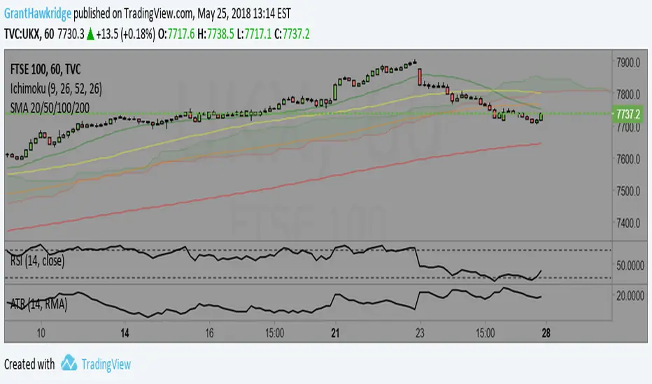
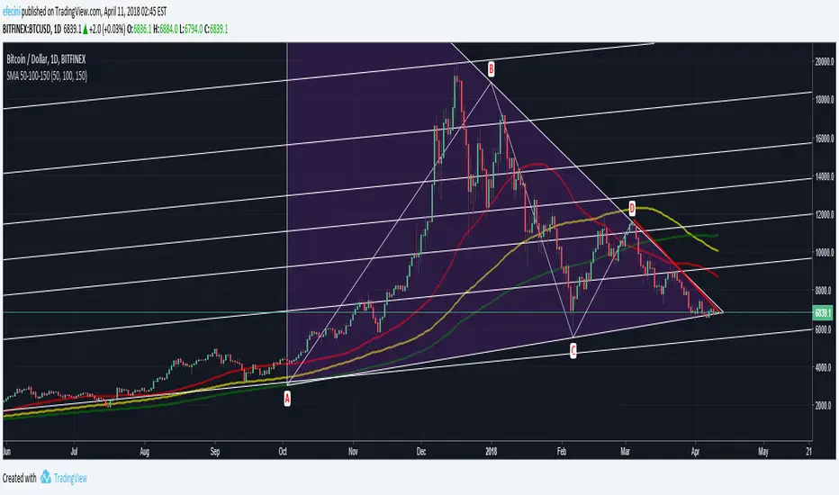
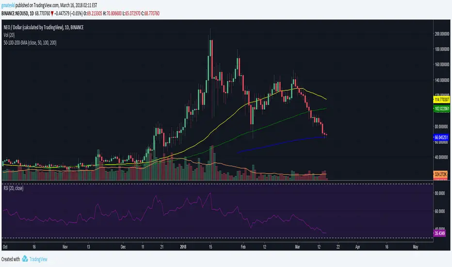
SMA 50/100 / 200Couldn't find a simple moving average that combined the three i was looking for so I made it. Nothing special.

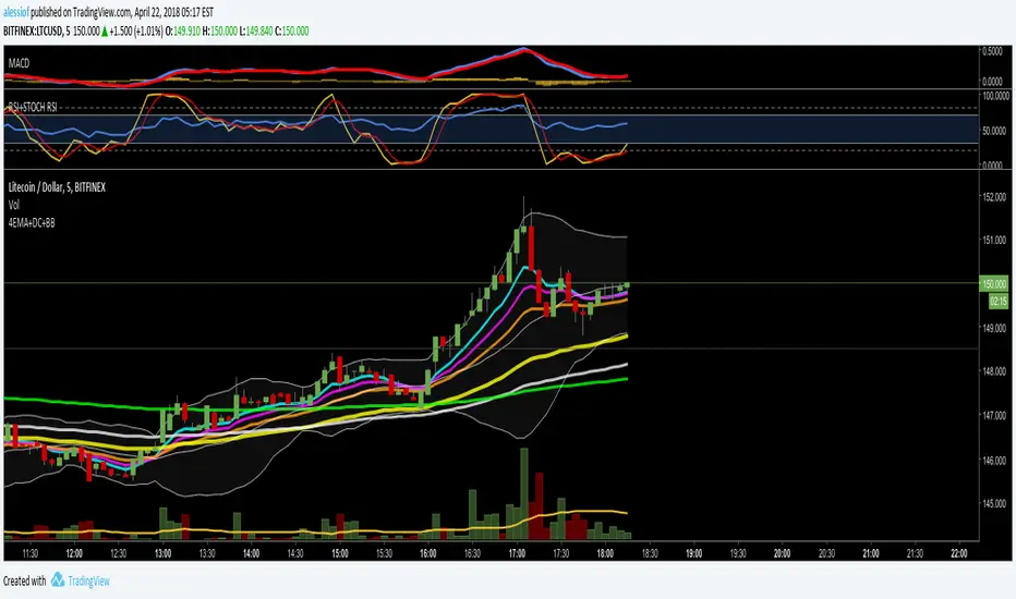
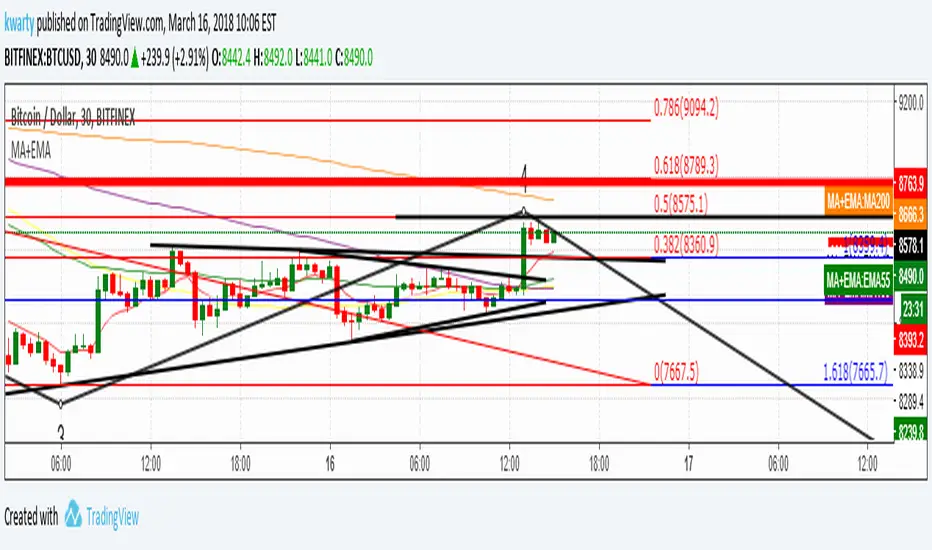
4EMA (8,13,21,55) + Death Cross (100,200) + Bollinger BandsUnited three indicators in one.
4 Moving Average Exponential: 8, 13, 21, 55 - as per @Philakone strategy
Moving Average Exponential - Death Cross: 100, 200
Bollinger Bands
Check out my other script for RSI and Stoch RSI all in one.
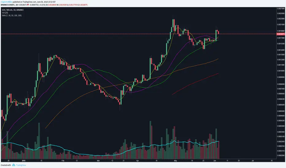
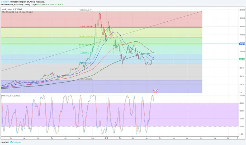
30, 50, 100 and 200 Day Simple Moving AveragesEasy to Use to see 30, 50, 100 and 200 Day Simple Moving Averages.
3xEMA 55 100 and 200the 55 blue 100 white and the 200 yellow EMA in one indicator uses current resolution time frame by default

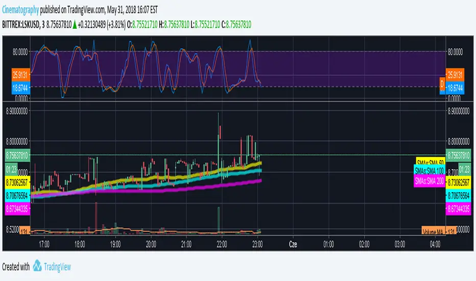
Moving Averages (10, 55, 100 EMAs, 200 SMA close)10, 55, 100 EMAs, 200 SMA close. Increasing line stroke, standard colors.

Philakone 55/100 EMA incl. color & sizeInspired on Philakone's EMA settings in his colors and line width. Also added 100 EMA.
Multiple Ema 20/50/100Multiple Ema 20/50/100 and you can add more EMA Plot easily by changing the codes.


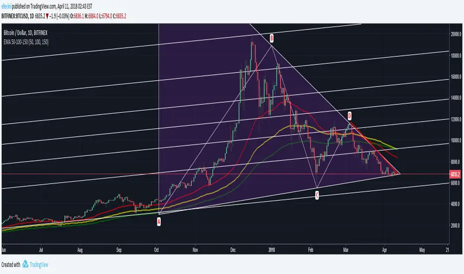
50, 100, 200 EMAsA simple script that displays the 50, 100, and 200-period exponential moving averages. Reduce clutter by combining them into one indicator!

50, 100, 200 SMAsA simple script that displays the 50, 100, and 200-period simple moving averages. Reduce clutter by combining them into one indicator!

50,100,200 MA by CryptoLife71(FIXED)Updated the code by CryptoLife71 so that the 200ma shows correctly.