Normalised Volume Oscillator [BackQuant]Normalised Volume Oscillator
A refined evolution of the Klinger Volume Oscillator, rebuilt for clarity, precision, and adaptability. This tool normalizes volume-driven momentum into a bounded scale so you can easily identify shifts in accumulation and distribution across any asset or timeframe, while keeping readings comparable between markets.
What this indicator does
The Normalised Volume Oscillator quantifies the balance between buying and selling pressure using the Klinger Volume Oscillator (KVO) as its base, then rescales it dynamically into a normalized range between -0.5 and +0.5. This normalization allows traders to interpret relative strength and exhaustion in volume flow, rather than dealing with raw unbounded values that differ across symbols.
It is a momentum-volume hybrid that reveals the strength of trend participation: when buyers dominate, normalized readings rise toward +0.5; when sellers dominate, they fall toward -0.5. The midline (0) acts as an equilibrium between accumulation and distribution.
Core components
Klinger Volume Oscillator: The foundation of this indicator, combining volume with price trend direction to measure long-term money flow relative to short-term movement.
Normalization process: The raw KVO is scaled over a user-defined Normalisation Period , computing `(KVO - lowest) / (highest - lowest) - 0.5`. This centers all readings around zero, allowing overbought/oversold detection independent of asset volatility or volume magnitude.
Signal moving average: The normalized KVO is smoothed with a user-selectable moving average type—SMA, EMA, DEMA, TEMA, HMA, ALMA, and others. This becomes the signal line for confirmation of trend direction or mean-reversion setups.
How it works conceptually
1. The KVO detects when volume supports price movement (bullish) or diverges from it (bearish).
2. The script normalizes the raw KVO so that relative magnitude is consistent—what is “strong buying pressure” looks the same on BTCUSD as it does on AAPL.
3. Overbought and oversold regions are derived statistically, rather than from arbitrary values, based on percentile zones around ±0.4 and ±0.5.
4. The oscillator is optionally combined with a moving average to help identify crossovers, momentum shifts, and divergence confirmation.
How to interpret it
Above 0: Indicates dominant buying pressure and likely continuation of upward momentum.
Below 0: Suggests dominant selling pressure and potential continuation of downward movement.
Crosses of 0: Often mark transitions between accumulation and distribution phases.
+0.4 to +0.5 zone: Overbought region where buying intensity is stretched; watch for deceleration or divergence.
[-0.4 to -0.5 zone: Oversold region indicating panic or exhaustion in selling.
Signal-line crossover: A traditional momentum confirmation method; when the normalized KVO crosses above its moving average, buyers regain control, and vice versa.
Why normalization matters
Typical volume oscillators are asset-specific—what is considered “high” volume for one symbol is not the same for another. By dynamically normalizing KVO values within a rolling lookback, this version transforms raw amplitude into a standardized scale. This means you can:
Compare multiple assets objectively.
Set consistent alert thresholds for overbought/oversold regions.
Avoid misleading interpretations from absolute oscillator values.
Customization and UI
Moving Average Type & Period: Select your preferred smoothing method (SMA, EMA, TEMA, etc.) and adjust its period to tune sensitivity.
Normalisation Period: Defines how many bars the KVO range is measured over; shorter periods adapt faster, longer ones smooth more.
Visual Toggles:
* Show Oscillator : enables or hides the core histogram.
* Show Moving Average : adds a smoothed overlay for signal confirmation.
* Paint Candles : optional color overlay for chart candles based on oscillator direction.
* Show Static Levels : displays ±0.4 and ±0.5 zones for overbought/oversold boundaries.
How to use it
Trend confirmation: Use midline (0) crossovers as confirmation of emerging trend shifts—cross above 0 suggests a new bullish phase, cross below 0 a bearish one.
Reversal spotting: Look for normalized readings reaching ±0.5 and flattening, or diverging against price extremes.
Divergence analysis: When price makes a new high but the normalized oscillator fails to, it signals waning buying conviction (and vice versa for lows).
Multi-timeframe integration: Works best alongside higher timeframe trend filters or moving averages; normalization makes this consistent.
Alerts
Prebuilt alert conditions allow quick automation:
Midline crossovers (0): transition between accumulation and distribution.
Overbought (+0.4) and Oversold (-0.4) triggers for potential exhaustion.
Signal moving-average crosses for confirmation entries.
Tips for use
Combine with price structure—don’t fade every overbought/oversold reading; confirm with break of structure or candle patterns.
Use longer normalization periods for position trading, shorter for intraday analysis.
In choppy markets, treat 0-line oscillations as noise filters, not trade triggers.
Summary
The Normalised Volume Oscillator modernizes the classic Klinger Volume Oscillator by normalizing its readings into a standardized range. This makes it more adaptive across assets and timeframes, improves interpretability, and provides intuitive, data-driven overbought/oversold levels. Whether used standalone or as a confirmation layer, it offers a clearer view of volume dynamics—revealing when markets are truly being accumulated, distributed, or stretched beyond their sustainable extremes.
M-oscillator

indicator CalibrationIndicator Calibration - Multi-Indicator Consensus System
Overview
Indicator Calibration is a powerful consensus-based trading indicator that leverages the MyIndicatorLibrary (NormalizedIndicators) to combine multiple trend-following indicators into a single, actionable signal. By averaging the normalized outputs of up to 8 different trend indicators, this tool provides traders with a clear consensus view of market direction, reducing noise and false signals inherent in single-indicator approaches.
The indicator outputs a value between -1 (strong bearish) and +1 (strong bullish), with 0 representing a neutral market state. This creates an intuitive, easy-to-read oscillator that synthesizes multiple analytical perspectives into one coherent signal.
🎯 Core Concept
Consensus Trading Philosophy
Rather than relying on a single indicator that may give conflicting or premature signals, Indicator Calibration employs a democratic voting system where multiple indicators contribute their normalized opinion:
Each enabled indicator votes: +1 (bullish), -1 (bearish), or 0 (neutral)
The votes are averaged to create a consensus signal
Strong consensus (closer to ±1) indicates high agreement among indicators
Weak consensus (closer to 0) indicates market indecision or transition
Key Benefits
Reduced False Signals: Multiple indicators must agree before strong signals appear
Noise Filtering: Individual indicator quirks are smoothed out by averaging
Customizable: Enable/disable indicators and adjust parameters to suit your trading style
Universal Application: Works across all timeframes and asset classes
Clear Visualization: Simple line oscillator with clear bull/bear zones
📊 Included Indicators
The system can utilize up to 8 normalized trend-following indicators from the library:
1. BBPct - Bollinger Bands Percent
Parameters: Length (default: 20), Factor (default: 2)
Type: Stationary oscillator
Strength: Mean reversion and volatility detection
2. NorosTrendRibbonEMA
Parameters: Length (default: 20)
Type: Non-stationary trend follower
Strength: Breakout detection with momentum confirmation
3. RSI - Relative Strength Index
Parameters: Length (default: 9), SMA Length (default: 4)
Type: Stationary momentum oscillator
Strength: Overbought/oversold with smoothing
4. Vidya - Variable Index Dynamic Average
Parameters: Length (default: 30), History Length (default: 9)
Type: Adaptive moving average
Strength: Volatility-adjusted trend following
5. HullSuite
Parameters: Length (default: 55), Multiplier (default: 1)
Type: Fast-response moving average
Strength: Low-lag trend identification
6. TrendContinuation
Parameters: MA Length 1 (default: 50), MA Length 2 (default: 25)
Type: Dual HMA system
Strength: Trend quality assessment with neutral states
7. LeonidasTrendFollowingSystem
Parameters: Short Length (default: 21), Key Length (default: 10)
Type: Dual EMA crossover
Strength: Simple, reliable trend tracking
8. TRAMA - Trend Regularity Adaptive Moving Average
Parameters: Length (default: 50)
Type: Adaptive trend follower
Strength: Adjusts to trend stability
⚙️ Input Parameters
Source Settings
Source: Choose your price input (default: close)
Can be modified to: open, high, low, close, hl2, hlc3, ohlc4, hlcc4
Indicator Selection
Each indicator can be enabled or disabled via checkboxes:
use_bbpct: Enable/disable Bollinger Bands Percent
use_noros: Enable/disable Noro's Trend Ribbon
use_rsi: Enable/disable RSI
use_vidya: Enable/disable VIDYA
use_hull: Enable/disable Hull Suite
use_trendcon: Enable/disable Trend Continuation
use_leonidas: Enable/disable Leonidas System
use_trama: Enable/disable TRAMA
Parameter Customization
Each indicator has its own parameter group where you can fine-tune:
val 1: Primary period/length parameter
val 2: Secondary parameter (multiplier, smoothing, etc.)
📈 Signal Interpretation
Output Line (Orange)
The main output oscillates between -1 and +1:
+1.0 to +0.5: Strong bullish consensus (all or most indicators agree on uptrend)
+0.5 to +0.2: Moderate bullish bias (bullish indicators outnumber bearish)
+0.2 to -0.2: Neutral zone (mixed signals or transition phase)
-0.2 to -0.5: Moderate bearish bias (bearish indicators outnumber bullish)
-0.5 to -1.0: Strong bearish consensus (all or most indicators agree on downtrend)
Reference Lines
Green line (+1): Maximum bullish consensus
Red line (-1): Maximum bearish consensus
Gray line (0): Neutral midpoint
💡 Trading Strategies
Strategy 1: Consensus Threshold Trading
Entry Rules:
- Long: Output crosses above +0.5 (strong bullish consensus)
- Short: Output crosses below -0.5 (strong bearish consensus)
Exit Rules:
- Exit Long: Output crosses below 0 (consensus lost)
- Exit Short: Output crosses above 0 (consensus lost)
Strategy 2: Zero-Line Crossover
Entry Rules:
- Long: Output crosses above 0 (bullish shift in consensus)
- Short: Output crosses below 0 (bearish shift in consensus)
Exit Rules:
- Exit on opposite crossover
Strategy 3: Divergence Trading
Look for divergences between:
- Price making higher highs while indicator makes lower highs (bearish divergence)
- Price making lower lows while indicator makes higher lows (bullish divergence)
Strategy 4: Extreme Reading Reversal
Entry Rules:
- Long: Output reaches -0.8 or below (extreme bearish consensus = potential reversal)
- Short: Output reaches +0.8 or above (extreme bullish consensus = potential reversal)
Use with caution - best combined with other reversal signals
🔧 Optimization Tips
For Trending Markets
Enable trend-following indicators: Noro's, VIDYA, Hull Suite, Leonidas
Use higher threshold levels (±0.6) to filter out minor retracements
Increase indicator periods for smoother signals
For Range-Bound Markets
Enable oscillators: BBPct, RSI
Use zero-line crossovers for entries
Decrease indicator periods for faster response
For Volatile Markets
Enable adaptive indicators: VIDYA, TRAMA
Use wider threshold levels to avoid whipsaws
Consider disabling fast indicators that may overreact
Custom Calibration Process
Start with all indicators enabled using default parameters
Backtest on your chosen timeframe and asset
Identify which indicators produce the most false signals
Disable or adjust parameters for problematic indicators
Test different threshold levels for entry/exit
Validate on out-of-sample data
📊 Visual Guide
Color Scheme
Orange Line: Main consensus output
Green Horizontal: Bullish extreme (+1)
Red Horizontal: Bearish extreme (-1)
Gray Horizontal: Neutral zone (0)
Reading the Chart
Line above 0: Net bullish sentiment
Line below 0: Net bearish sentiment
Line near extremes: Strong consensus
Line fluctuating near 0: Indecision or transition
Smooth line movement: Stable consensus
Erratic line movement: Conflicting signals
⚠️ Important Considerations
Lag Characteristics
This is a lagging indicator by design (consensus takes time to form)
Best used for trend confirmation rather than early entry
May miss the first portion of strong moves
Reduces false entries at the cost of delayed entries
Number of Active Indicators
More indicators = smoother but slower signals
Fewer indicators = faster but potentially noisier signals
Minimum recommended: 4 indicators for reliable consensus
Optimal: 6-8 indicators for balanced performance
Market Conditions
Best: Strong trending markets (up or down)
Good: Volatile markets with clear directional moves
Poor: Choppy, sideways markets with no clear trend
Worst: Low-volume, range-bound conditions
Complementary Tools
Consider combining with:
Volume analysis for confirmation
Support/resistance levels for entry/exit points
Market structure analysis (higher timeframe trends)
Risk management tools (ATR-based stops)
🎓 Example Use Cases
Swing Trading
Timeframe: Daily or 4H
Enable: All 8 indicators with default parameters
Entry: Consensus > +0.5 or < -0.5
Hold: Until consensus reverses to opposite extreme
Day Trading
Timeframe: 15m or 1H
Enable: Faster indicators (RSI, BBPct, Noro's, Hull Suite)
Entry: Zero-line crossover with volume confirmation
Exit: Opposite crossover or profit target
Position Trading
Timeframe: Weekly or Daily
Enable: Slower indicators (TRAMA, VIDYA, Trend Continuation)
Entry: Strong consensus (±0.7) with higher timeframe confirmation
Hold: Months until consensus weakens significantly
🔬 Technical Details
Calculation Method
1. Each enabled indicator calculates its normalized signal (-1, 0, or +1)
2. All active signals are stored in an array
3. Array.avg() computes the arithmetic mean
4. Result is plotted as a continuous line
Output Range
Theoretical: -1.0 to +1.0
Practical: Typically ranges between -0.8 to +0.8
Rare: All indicators perfectly aligned at ±1.0
Performance
Lightweight calculation (simple averaging)
No repainting (all indicators are non-repainting)
Compatible with all Pine Script features
Works on all TradingView plans
📋 License
This code is subject to the Mozilla Public License 2.0 at mozilla.org
🚀 Quick Start Guide
Add to Chart: Apply indicator to your chart
Choose Timeframe: Select appropriate timeframe for your trading style
Enable Indicators: Start with all 8 enabled
Observe Behavior: Watch how consensus forms during different market conditions
Calibrate: Adjust parameters and indicator selection based on observations
Backtest: Validate your settings on historical data
Trade: Apply with proper risk management
🎯 Key Takeaways
✅ Consensus beats individual indicators - Multiple perspectives reduce errors
✅ Customizable to your style - Enable/disable and tune to preference
✅ Simple interpretation - One line tells the story
✅ Works across markets - Stocks, crypto, forex, commodities
✅ Reduces emotional trading - Clear, objective signal generation
✅ Professional-grade - Built on proven technical analysis principles
Indicator Calibration transforms complex multi-indicator analysis into a single, actionable signal. By harnessing the collective wisdom of multiple proven trend-following systems, traders gain a powerful edge in identifying high-probability trade setups while filtering out market noise.

Smart RSI Money Flow - Core Bands V1.01SMART RSI – Money Flow Bands (Technical Overview)
1. Background: RSI and Its Behavior on Lower Timeframes
The Relative Strength Index (RSI) originally is a momentum oscillator calculated from average gains and losses over a selected period. In its standard form, RSI is derived solely from price changes; it does not incorporate volume data or order-flow information in its formula.
Because RSI is price-based, its interpretation depends strongly on the timeframe:
• On higher timeframes, each bar aggregates more trading activity, and RSI tends to behave more smoothly.
• On lower timeframes (1-hour down to intraday scalping intervals), price fluctuations are quicker, and RSI becomes more sensitive to short-term noise.
This does not imply that RSI becomes invalid, but that its signals on fast charts can be more reactive and may benefit from additional context such as volume behavior or structural information.
2. Purpose of This Indicator
This indicator extends the classical RSI by adding information that RSI does not include:
• Mapping RSI values into price-based bands instead of the 0–100 oscillator space.
• Retrieving lower timeframe volume data and separating it into buy and sell components.
• Comparing the slope (angle) of price movement with the slope of buy and sell volume.
The goal is to provide a structural interpretation of where price sits relative to RSI conditions and how volume is behaving on a lower timeframe.
3. Technical Differences Compared to Classical RSI
A) Classical RSI
• Input: price only (usually close).
• Output: normalized oscillator between 0 and 100.
• Does not incorporate intra-bar volume distribution.
• Does not separate buy/sell volume.
B) SMART RSI – Money Flow Bands
1) RSI-to-Price Mapping
Converts RSI values into upper/lower price bands using recent price extremes.
2) Lower Timeframe Volume Decomposition
Retrieves LTF data and splits each bar’s volume into buy (close>open) and sell (close

TASC 2025.12 The One Euro Filter█ OVERVIEW
This script implements the One Euro filter, developed by Georges Casiez, Nicolas Roussel, and Daniel Vogel, and adapted by John F. Ehlers in his article "Low-Latency Smoothing" from the December 2025 edition of the TASC Traders' Tips . The original creators gave the filter its name to suggest that it is cheap and efficient, like something one might purchase for a single Euro.
█ CONCEPTS
The One Euro filter is an EMA-based low-pass filter that adapts its smoothing factor (alpha) based on the absolute values of smoothed rates of change in the source series. It was designed to filter noisy, high-frequency signals in real time with low latency. Ehlers simplifies the filter for market analysis by calculating alpha in terms of bar periods rather than time and frequency, because periods are naturally intuitive for a discrete financial time series.
In his article, Ehlers demonstrates how traders can apply the adaptive One Euro filter to a price series for simple low-latency smoothing. Additionally, he explains that traders can use the filter as a smoothed oscillator by applying it to a high-pass filter. In essence, similar to other low-pass filters, traders can apply the One Euro filter to any custom source to derive a smoother signal with reduced noise and low lag.
This script applies the One Euro filter to a specified source series, and it applies the filter to a two-pole high-pass filter or other oscillator, depending on the selected "Osc type" option. By default, it displays the filtered source series on the main chart pane, and it shows the oscillator and its filtered series in a separate pane.
█ INPUTS
Source: The source series for the first filter and the selected oscillator.
Min period: The minimum cutoff period for the smoothing calculation.
Beta: Controls the responsiveness of the filter. The filter adds the product of this value and the smoothed source change to the minimum period to determine the filter's smoothing factor. Larger values cause more significant changes in the maximum cutoff period, resulting in a smoother response.
Osc type: The type of oscillator to calculate for the pane display. By default, the indicator calculates a high-pass filter. If the selected type is "None", the indicator displays the "Source" series and its filtered result in a separate pane rather than showing the filter on the main chart. With this setting, users can pass plotted values from another indicator and view the filtered result in the pane.
Period: The length for the selected oscillator's calculation.

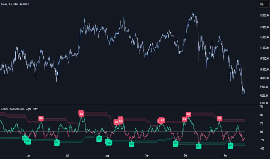
Baseline Deviation Oscillator [Alpha Extract]A sophisticated normalized oscillator system that measures price deviation from a customizable moving average baseline using ATR-based scaling and dynamic threshold adaptation. Utilizing advanced HL median filtering and multi-timeframe threshold calculations, this indicator delivers institutional-grade overbought/oversold detection with automatic zone adjustment based on recent oscillator extremes. The system's flexible baseline architecture supports six different moving average types while maintaining consistent ATR normalization for reliable signal generation across varying market volatility conditions.
🔶 Advanced Baseline Construction Framework
Implements flexible moving average architecture supporting EMA, RMA, SMA, WMA, HMA, and TEMA calculations with configurable source selection for optimal baseline customization. The system applies HL median filtering to the raw baseline for exceptional smoothing and outlier resistance, creating ultra-stable trend reference levels suitable for precise deviation measurement.
// Flexible Baseline MA System
ma(src, length, type) =>
if type == "EMA"
ta.ema(src, length)
else if type == "TEMA"
ema1 = ta.ema(src, length)
ema2 = ta.ema(ema1, length)
ema3 = ta.ema(ema2, length)
3 * ema1 - 3 * ema2 + ema3
// Baseline with HL Median Smoothing
Baseline_Raw = ma(src, MA_Length, MA_Type)
Baseline = hlMedian(Baseline_Raw, HL_Filter_Length)
🔶 ATR Normalization Engine
Features sophisticated ATR-based scaling methodology that normalizes price deviations relative to current volatility conditions, ensuring consistent oscillator readings across different market regimes. The system calculates ATR bands around the baseline and uses half the band width as the normalization factor for volatility-adjusted deviation measurement.
🔶 Dynamic Threshold Adaptation System
Implements intelligent threshold calculation using rolling window analysis of oscillator extremes with configurable smoothing and expansion parameters. The system identifies peak and trough levels over dynamic windows, applies EMA smoothing, and adds expansion factors to create adaptive overbought/oversold zones that adjust to changing market conditions.
1D
3D
1W
🔶 Multi-Source Configuration Architecture
Provides comprehensive source selection including Close, Open, HL2, HLC3, and OHLC4 options for baseline calculation, enabling traders to optimize oscillator behavior for specific trading styles. The flexible source system allows adaptation to different market characteristics while maintaining consistent ATR normalization methodology.
🔶 Signal Generation Framework
Generates bounce signals when oscillator crosses back through dynamic thresholds and zero-line crossover signals for trend confirmation. The system identifies both standard threshold bounces and extreme zone bounces with distinct alert conditions for comprehensive reversal and continuation pattern detection.
Bull_Bounce = ta.crossover(OSC, -Active_Lower) or
ta.crossover(OSC, -Active_Lower_Extreme)
Bear_Bounce = ta.crossunder(OSC, Active_Upper) or
ta.crossunder(OSC, Active_Upper_Extreme)
// Zero Line Signals
Zero_Cross_Up = ta.crossover(OSC, 0)
Zero_Cross_Down = ta.crossunder(OSC, 0)
🔶 Enhanced Visual Architecture
Provides color-coded oscillator line with bullish/bearish dynamic coloring, signal line overlay for trend confirmation, and optional cloud fills between oscillator and signal. The system includes gradient zone fills for overbought/oversold regions with configurable transparency and threshold level visualization with automatic label generation.
snapshot
🔶 HL Median Filter Integration
Features advanced high-low median filtering identical to DEMA Flow for exceptional baseline smoothing without lag introduction. The system constructs rolling windows of baseline values, performs median extraction for both odd and even window lengths, and eliminates outliers for ultra-clean deviation measurement baseline.
🔶 Comprehensive Alert System
Implements multi-tier alert framework covering bullish bounces from oversold zones, bearish bounces from overbought zones, and zero-line crossovers in both directions. The system provides real-time notifications for critical oscillator events with customizable message templates for automated trading integration.
🔶 Performance Optimization Framework
Utilizes efficient calculation methods with optimized array management for median filtering and minimal computational overhead for real-time oscillator updates. The system includes intelligent null value handling and automatic scale factor protection to prevent division errors during extreme market conditions.
🔶 Why Choose Baseline Deviation Oscillator ?
This indicator delivers sophisticated normalized oscillator analysis through flexible baseline architecture and dynamic threshold adaptation. Unlike traditional oscillators with fixed levels, the BDO automatically adjusts overbought/oversold zones based on recent oscillator behavior while maintaining consistent ATR normalization for reliable cross-market and cross-timeframe comparison. The system's combination of multiple MA type support, HL median filtering, and intelligent zone expansion makes it essential for traders seeking adaptive momentum analysis with reduced false signals and comprehensive reversal detection across cryptocurrency, forex, and equity markets.
Frequency Momentum Oscillator [QuantAlgo]🟢 Overview
The Frequency Momentum Oscillator applies Fourier-based spectral analysis principles to price action to identify regime shifts and directional momentum. It calculates Fourier coefficients for selected harmonic frequencies on detrended price data, then measures the distribution of power across low, mid, and high frequency bands to distinguish between persistent directional trends and transient market noise. This approach provides traders with a quantitative framework for assessing whether current price action represents meaningful momentum or merely random fluctuations, enabling more informed entry and exit decisions across various asset classes and timeframes.
🟢 How It Works
The calculation process removes the dominant trend from price data by subtracting a simple moving average, isolating cyclical components for frequency analysis:
detrendedPrice = close - ta.sma(close , frequencyPeriod)
The detrended price series undergoes frequency decomposition through Fourier coefficient calculation across the first 8 harmonics. For each harmonic frequency, the algorithm computes sine and cosine components across the lookback window, then derives power as the sum of squared coefficients:
for k = 1 to 8
cosSum = 0.0
sinSum = 0.0
for n = 0 to frequencyPeriod - 1
angle = 2 * math.pi * k * n / frequencyPeriod
cosSum := cosSum + detrendedPrice * math.cos(angle)
sinSum := sinSum + detrendedPrice * math.sin(angle)
power = (cosSum * cosSum + sinSum * sinSum) / frequencyPeriod
Power measurements are aggregated into three frequency bands: low frequencies (harmonics 1-2) capturing persistent cycles, mid frequencies (harmonics 3-4), and high frequencies (harmonics 5-8) representing noise. Each band's power normalizes against total spectral power to create percentage distributions:
lowFreqNorm = totalPower > 0 ? (lowFreqPower / totalPower) * 100 : 33.33
highFreqNorm = totalPower > 0 ? (highFreqPower / totalPower) * 100 : 33.33
The normalized frequency components undergo exponential smoothing before calculating spectral balance as the difference between low and high frequency power:
smoothLow = ta.ema(lowFreqNorm, smoothingPeriod)
smoothHigh = ta.ema(highFreqNorm, smoothingPeriod)
spectralBalance = smoothLow - smoothHigh
Spectral balance combines with price momentum through directional multiplication, producing a composite signal that integrates frequency characteristics with price direction:
momentum = ta.change(close , frequencyPeriod/2)
compositeSignal = spectralBalance * math.sign(momentum)
finalSignal = ta.ema(compositeSignal, smoothingPeriod)
The final signal oscillates around zero, with positive values indicating low-frequency dominance coupled with upward momentum (trending up), and negative values indicating either high-frequency dominance (choppy market) or downward momentum (trending down).
🟢 How to Use This Indicator
→ Long/Short Signals: the indicator generates long signals when the smoothed composite signal crosses above zero (indicating low-frequency directional strength dominates) and short signals when it crosses below zero (indicating bearish momentum persistence).
→ Upper and Lower Reference Lines: the +25 and -25 reference lines serve as threshold markers for momentum strength. Readings beyond these levels indicate strong directional conviction, while oscillations between them suggest consolidation or weakening momentum. These references help traders distinguish between strong trending regimes and choppy transitional periods.
→ Preconfigured Presets: three optimized configurations are available with Default (32, 3) offering balanced responsiveness, Fast Response (24, 2) designed for scalping and intraday trading, and Smooth Trend (40, 5) calibrated for swing trading and position trading with enhanced noise filtration.
→ Built-in Alerts: the indicator includes three alert conditions for automated monitoring - Long Signal (momentum shifts bullish), Short Signal (momentum shifts bearish), and Signal Change (any directional transition). These alerts enable traders to receive real-time notifications without continuous chart monitoring.
→ Color Customization: four visual themes (Classic green/red, Aqua blue/orange, Cosmic aqua/purple, Custom) allow chart customization for different display environments and personal preferences.

GTI - Overbought and Oversold indicatorFor this indicator I've merged 6 indicators (RSI, Stochastic, CCI, MFI, UO and William %R) that are decent to spot overbought and oversold conditions into one indicator.
The idea is the more indicators that agree on overbought and oversold conditions, the better chance that the condition is correct.
Possible input settings
Set your own values for the overbought and oversold bands.
Noise suppression (On/Off)
Length for noise suppression calculations
Overbought noise suppression
Oversold noise suppression
Plot divergences (On/Off)
Left/Right lookback settings for finding pivot highs/lows
Min/Max lookback range to compare pivots for divergences
Style settings
Enabled/Disable the line for reversal value
Set the color for the line (default is 100% transparent value)
Enable/Disable fill color between reversal value and the 0 line
Set the fill color
Precision for reversal value, default is 2
Explanations
The scale goes from 100 to -100, where outliners above 85 or below -85 is expected to be extremely rare. The overbought and oversold bands are calculated from the typical values from each indicator used in the calculation.
The noise suppression is a percentile calculation from the last X bars back, where X is the length you set in the settings. 100 is the default value. This is very good to use in strong trends as an asset in a strong bullish trend tend to not touch/breach the oversold band and vise versa. The percentile calculation might still be able to catch the overbought/oversold condition in a strong opposite trending asset. 85 is a default value, but keep in mind that every asset moves differently due to their liquidity pool. The default is only a guide line.
The divergence settings only plots normal divergences. Hidden divergences are not calculated.
If you want the possibility to plot/see hidden divergences too, let me know in the comments. If enough people wants it I'll consider adding them.
when it comes to the style, you might be a bit confused at first. The reversal value is enabled, but not showing. That's because it's enabled with 100% transparency as I like using the fill more than just a line.
If you want to use a line instead of the fill, Disable the fill -> edit reversal value color -> set your chosen color and make sure to remove the transparency to make it visible.
Exmaple, ticker NOVO_B
In the example ticker I've enabled "Noise suppression", using the default 100 length and set noise suppression for both OB and OS to 90.
The green and red circles are plotted when the "reversal value" falls below the percentile set, indicating that a possible top was just formed.
Keep in mind that strong bullish or bearish trends tend to stay overbought/oversold for a longer time and are likely to print several false signals before the eventual reversal. If a divergences is printed, normally that is either the bottom or close to the bottom before a stronger reversal.
Suggestion
As all other indicators, don't use this indicator alone to spot reversals. Use it together with 1-3 other indicators like MACD, ADX and OBV. I like to use MACD as a confirmation tool after this tool starts indicating overbought/oversold conditions.
For an overbought condition, wait for MACD to cross below the signal line.
For an oversold condition, wait for the MACD to cross above the signal line.
This way you don't act on false signal.
Another way would be to use a DCA strategy, where you buy on each signal. In such a situation I suggest starting small enough to be able to double the total for each time, example below.
First signal: $100, then another $100 on second signal, $200 on third signal, $400 on fourth signal and so on. The amounts are an example, find what works for you.


Known Reversals (CreativeAdvance)1 min left to edit script
13 minutes ago
Known Reversals (CreativeAdvance)
Manage access
Add to favorites
Use on chart
0
0
Known Reversals
Non-repainting 1-bar reversal detector
What it does:
Pinpoints the earliest confirmed reversals by detecting a subtle divergence within prevailing momentum. Delivers signals with zero lag and no repaint.
Core logic:
- Monitors directional momentum via highs in uptrends and lows in downtrends
- Activates only when the **close breaks alignment** with that momentum in a single candle
- Proprietary volatility-adjusted oscillator ensures signals fire exclusively in high-probability reversal contexts
Key advantage:
Reveals lower-timeframe reversals the moment they confirm on the current chart — true X-ray vision for precision entries.
Pro tip:
Use with distinct candlestick outline colors to instantly distinguish bullish vs. bearish signals, especially on inside bar reversals (painted uniformly for clarity).
No inputs. No curve-fitting. Just pure, actionable reversal confirmation.

CandelaCharts - Trend Oscillator 📝 Overview
Trend Oscillator is a simple yet effective trend identification tool that uses the relationship between two exponential moving averages (EMAs) to determine market direction. It calculates the spread between a fast and slow EMA, applies a bias multiplier, and smooths the result to produce a clean oscillator that oscillates above and below a zero line. When the oscillator is above zero, the trend is considered bullish (upward); when below zero, it's bearish (downward). The indicator provides clear visual feedback through color-coded plots and optional price bar coloring, making it easy to identify trend direction at a glance.
📦 Features
This section highlights the core capabilities you'll rely on most.
Dual EMA system — Uses a fast EMA (default 9) and slow EMA (default 21) to capture trend momentum and direction.
Bias multiplier — Applies a small multiplier (default 1.001) to the EMA spread, providing a slight bias that helps filter noise and confirm trend strength.
Smoothed output — Applies an additional EMA smoothing (default 5 periods) to the raw spread, creating a cleaner, less choppy oscillator line.
Zero-line reference — Plots a horizontal zero line that serves as the critical threshold between bullish and bearish conditions.
Color-coded visualization — Automatically colors the oscillator line green/lime when bullish (above zero) and red when bearish (below zero).
Price bar coloring — Optional feature to color price bars based on the current trend direction, providing immediate visual context on the main chart.
Customizable parameters — Adjust EMA lengths, bias multiplier, smoothing period, and colors to match your trading style and timeframe.
⚙️ Settings
Use these controls to fine-tune the oscillator's sensitivity, appearance, and behavior.
Fast EMA Length — Period for the fast exponential moving average (default: 9). Lower values make the indicator more responsive to price changes.
Slow EMA Length — Period for the slow exponential moving average (default: 21). Higher values create a smoother baseline for trend identification.
Bias Multiplier — Multiplier applied to the EMA spread (default: 1.001). Small adjustments can help filter minor whipsaws and confirm trend strength.
Smoothing Length — Period for smoothing the raw spread calculation (default: 5). Higher values create a smoother oscillator line but may lag price action.
Colors — Set the bullish (default: lime) and bearish (default: red) colors for the oscillator line.
Color Price Bars — Toggle to enable/disable coloring of price bars based on the current trend direction.
⚡️ Showcase
Oscillator Line
Bar Coloring
Divergences
📒 Usage
Follow these steps to effectively use Trend Oscillator for trend identification and trading decisions.
1) Select your timeframe — The indicator works across all timeframes, but higher timeframes (daily, weekly, monthly) typically provide more reliable trend signals with less noise. Lower timeframes (1m, 5m, 15m) may produce more frequent but potentially less reliable signals. Consider your trading style: swing traders benefit from daily/weekly charts, while day traders can use 15m/1h timeframes. Always align the indicator's sensitivity with your timeframe choice.
2) Adjust EMA lengths — The default 9/21 combination works well for most cases. For faster signals, try 5/13; for slower, more conservative signals, try 12/26 or 20/50. Match the lengths to your trading style and timeframe.
3) Interpret the zero line — When the oscillator is above zero (green/lime), the trend is bullish. When below zero (red), the trend is bearish. The further from zero, the stronger the trend.
4) Watch for crossovers — Trend changes occur when the oscillator crosses the zero line. A cross from below to above indicates a shift to bullish; from above to below indicates a shift to bearish.
5) Identify divergences — Divergences can signal potential trend reversals. Bullish divergence : price makes lower lows while the oscillator makes higher lows (suggests weakening bearish momentum). Bearish divergence : price makes higher highs while the oscillator makes lower highs (suggests weakening bullish momentum). Divergences are most reliable when they occur near extreme levels and should be confirmed with price action before taking trades.
6) Use smoothing wisely — The smoothing parameter helps reduce noise but adds lag. Lower smoothing (3-5) is more responsive; higher smoothing (7-10) is more stable but slower to react.
7) Combine with price action — Use the oscillator to confirm trend direction, then look for entry opportunities when price pulls back in the direction of the trend. The optional price bar coloring helps visualize trend alignment on the main chart.
8) Filter with bias multiplier — The bias multiplier can help reduce false signals. Experiment with values between 1.000 and 1.005 to find the sweet spot for your instrument and timeframe.
🚨 Alerts
There are no built-in alerts in this version.
⚠️ Disclaimer
Trading involves significant risk, and many participants may incur losses. The content on this site is not intended as financial advice and should not be interpreted as such. Decisions to buy, sell, hold, or trade securities, commodities, or other financial instruments carry inherent risks and are best made with guidance from qualified financial professionals. Past performance is not indicative of future results.

Average True Range with MAKey features
ATR calculation: true range (ta.tr(true)) is smoothed using a selectable method to produce the ATR.
ATR smoothing options: RMA, SMA, EMA, or WMA for the ATR calculation.
MA-on-ATR: a separate moving average computed on the ATR values with its own length and smoothing method.
Display controls: toggles to show/hide the ATR and the ATR MA independently.
Appearance controls: separate color inputs for the ATR and the ATR MA, and a thicker line for the MA (linewidth=2).
Inputs
ATR Length (default 14): length used to smooth true range into the ATR.
ATR Smoothing (default RMA): smoothing method applied to the true range to form ATR.
MA Length (on ATR) (default 14): length for the moving average applied to the ATR series.
MA Smoothing (default SMA): smoothing method used for the MA applied to ATR.
Show ATR / Show ATR MA: booleans to toggle visibility.
ATR Color / ATR MA Color: choose plot colors.
How to interpret
ATR line: shows current volatility (average true range). Rising ATR indicates increasing volatility; falling ATR indicates decreasing volatility.
ATR MA line: smooths the ATR to reveal trend direction and reduce noise.
Use crossovers: ATR crossing above its MA may signal volatility is picking up; ATR crossing below its MA suggests volatility is subsiding.
Combine with price action or other indicators (e.g., breakout systems, position sizing rules) to make decisions based on volatility regime.
hell 1good for finding tops and bottoms in a trend .set to log scale and strech it like it looks in the chart
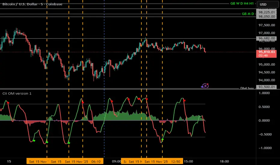
CII OM version 1CII OM Version 1 is a comprehensive trading indicator designed to provide a clear view of market momentum, money flow, and potential reversals in one subwindow. It combines multiple technical tools and visual cues to help traders identify high-probability reversal areas.
Features:
1. Chaikin Money Flow (CMF)
a. Measures buying and selling pressure over a period (default 20).
b. Positive CMF values are filled in green, negative in red.
c. Visualizes money flow for better context of market strength.
2. Volume Buy/Sell % (Optional)
a. Displays the proportion of buying versus selling volume per bar.
b. Green columns represent buying volume, red columns represent selling volume.
c. Can be enabled or disabled via the settings (default: off).
3. Stochastic Oscillator with Combined %K/%D Line
a. %K and %D lines combined into a single line for simplicity.
b. Green line indicates %K above %D (bullish), red line indicates %K below %D (bearish).
c. Upper/lower thresholds are marked at ±0.6.
d. Reversal zones are filled in aqua (buy zone) and fuchsia (sell zone).
4. Reversal Dots
a. Large dots indicate the end of a bullish or bearish reversal zone based on stochastic thresholds.
b. Smaller dots mark minor threshold crossings at ±0.6 for early detection of potential reversals.
c. Dot size is adjustable.
5. Ultimate Oscillator (Optional)
a. Measures short, medium, and long-term momentum.
b. Can be toggled on/off via the settings (default: off).
Customization Options:
a. Enable/disable Buy/Sell Volume % bars
b. Enable/disable Ultimate Oscillator
c. Adjust main reversal dot size
Adjust stochastic oscillator periods (K, D, smooth)
a. Fully compatible with Pine Script v5

Algorithm Predator - ProAlgorithm Predator - Pro: Advanced Multi-Agent Reinforcement Learning Trading System
Algorithm Predator - Pro combines four specialized market microstructure agents with a state-of-the-art reinforcement learning framework . Unlike traditional indicator mashups, this system implements genuine machine learning to automatically discover which detection strategies work best in current market conditions and adapts continuously without manual intervention.
Core Innovation: Rather than forcing traders to interpret conflicting signals, this system uses 15 different multi-armed bandit algorithms and a full reinforcement learning stack (Q-Learning, TD(λ) with eligibility traces, and Policy Gradient with REINFORCE) to learn optimal agent selection policies. The result is a self-improving system that gets smarter with every trade.
Target Users: Swing traders, day traders, and algorithmic traders seeking systematic signal generation with mathematical rigor. Suitable for stocks, forex, crypto, and futures on liquid instruments (>100k daily volume).
Why These Components Are Combined
The Fundamental Problem
No single indicator works consistently across all market regimes. What works in trending markets fails in ranging conditions. Traditional solutions force traders to manually switch indicators (slow, error-prone) or interpret all signals simultaneously (cognitive overload).
This system solves the problem through automated meta-learning: Deploy multiple specialized agents designed for specific market microstructure conditions, then use reinforcement learning to discover which agent (or combination) performs best in real-time.
Why These Specific Four Agents?
The four agents provide orthogonal failure mode coverage —each agent's weakness is another's strength:
Spoofing Detector - Optimal in consolidation/manipulation; fails in trending markets (hedged by Exhaustion Detector)
Exhaustion Detector - Optimal at trend climax; fails in range-bound markets (hedged by Liquidity Void)
Liquidity Void - Optimal pre-breakout compression; fails in established trends (hedged by Mean Reversion)
Mean Reversion - Optimal in low volatility; fails in strong trends (hedged by Spoofing Detector)
This creates complete market state coverage where at least one agent should perform well in any condition. The bandit system identifies which one without human intervention.
Why Reinforcement Learning vs. Simple Voting?
Traditional consensus systems have fatal flaws: equal weighting assumes all agents are equally reliable (false), static thresholds don't adapt, and no learning means past mistakes repeat indefinitely.
Reinforcement learning solves this through the exploration-exploitation tradeoff: Continuously test underused agents (exploration) while primarily relying on proven winners (exploitation). Over time, the system builds a probability distribution over agent quality reflecting actual market performance.
Mathematical Foundation: Multi-armed bandit problem from probability theory, where each agent is an "arm" with unknown reward distribution. The goal is to maximize cumulative reward while efficiently learning each arm's true quality.
The Four Trading Agents: Technical Explanation
Agent 1: 🎭 Spoofing Detector (Institutional Manipulation Detection)
Theoretical Basis: Market microstructure theory on order flow toxicity and information asymmetry. Based on research by Easley, López de Prado, and O'Hara on high-frequency trading manipulation.
What It Detects:
1. Iceberg Orders (Hidden Liquidity Absorption)
Method: Monitors volume spikes (>2.5× 20-period average) with minimal price movement (<0.3× ATR)
Formula: score += (close > open ? -2.5 : 2.5) when volume > vol_avg × 2.5 AND abs(close - open) / ATR < 0.3
Interpretation: Large volume without price movement indicates institutional absorption (buying) or distribution (selling) using hidden orders
Signal Logic: Contrarian—fade false breakouts caused by institutional manipulation
2. Spoofing Patterns (Fake Liquidity via Layering)
Method: Analyzes candlestick wick-to-body ratios during volume spikes
Formula: if upper_wick > body × 2 AND volume_spike: score += 2.0
Mechanism: Spoofing creates large wicks (orders pulled before execution) with volume evidence
Signal Logic: Wick direction indicates trapped participants; trade against the failed move
3. Post-Manipulation Reversals
Method: Tracks volume decay after manipulation events
Formula: if volume > vol_avg × 3 AND volume / volume < 0.3: score += (close > open ? -1.5 : 1.5)
Interpretation: Sharp volume drop after manipulation indicates exhaustion of manipulative orders
Why It Works: Institutional manipulation creates detectable microstructure anomalies. While retail traders see "mysterious reversals," this agent quantifies the order flow patterns causing them.
Parameter: i_spoof (sensitivity 0.5-2.0) - Controls detection threshold
Best Markets: Consolidations before breakouts, London/NY overlap windows, stocks with institutional ownership >70%
Agent 2: ⚡ Exhaustion Detector (Momentum Failure Analysis)
Theoretical Basis: Technical analysis divergence theory combined with VPIN reversals from market microstructure literature.
What It Detects:
1. Price-RSI Divergence (Momentum Deceleration)
Method: Compares 5-bar price ROC against RSI change
Formula: if price_roc > 5% AND rsi_current < rsi : score += 1.8
Mathematics: Second derivative detecting inflection points
Signal Logic: When price makes higher highs but momentum makes lower highs, expect mean reversion
2. Volume Exhaustion (Buying/Selling Climax)
Method: Identifies strong price moves (>5% ROC) with declining volume (<-20% volume ROC)
Formula: if price_roc > 5 AND vol_roc < -20: score += 2.5
Interpretation: Price extension without volume support indicates retail chasing while institutions exit
3. Momentum Deceleration (Acceleration Analysis)
Method: Compares recent 3-bar momentum to prior 3-bar momentum
Formula: deceleration = abs(mom1) < abs(mom2) × 0.5 where momentum significant (> ATR)
Signal Logic: When rate of price change decelerates significantly, anticipate directional shift
Why It Works: Momentum is lagging, but momentum divergence is leading. By comparing momentum's rate of change to price, this agent detects "weakening conviction" before reversals become obvious.
Parameter: i_momentum (sensitivity 0.5-2.0)
Best Markets: Strong trends reaching climax, parabolic moves, instruments with high retail participation
Agent 3: 💧 Liquidity Void Detector (Breakout Anticipation)
Theoretical Basis: Market liquidity theory and order book dynamics. Based on research into "liquidity holes" and volatility compression preceding expansion.
What It Detects:
1. Bollinger Band Squeeze (Volatility Compression)
Method: Monitors Bollinger Band width relative to 50-period average
Formula: bb_width = (upper_band - lower_band) / middle_band; triggers when < 0.6× average
Mathematical Foundation: Regression to the mean—low volatility precedes high volatility
Signal Logic: When volatility compresses AND cumulative delta shows directional bias, anticipate breakout
2. Volume Profile Gaps (Thin Liquidity Zones)
Method: Identifies sharp volume transitions indicating few limit orders
Formula: if volume < vol_avg × 0.5 AND volume < vol_avg × 0.5 AND volume > vol_avg × 1.5
Interpretation: Sudden volume drop after spike indicates price moved through order book to low-opposition area
Signal Logic: Price accelerates through low-liquidity zones
3. Stop Hunts (Liquidity Grabs Before Reversals)
Method: Detects new 20-bar highs/lows with immediate reversal and rejection wick
Formula: if new_high AND close < high - (high - low) × 0.6: score += 3.0
Mechanism: Market makers push price to trigger stop-loss clusters, then reverse
Signal Logic: Enter reversal after stop-hunt completes
Why It Works: Order book theory shows price moves fastest through zones with minimal liquidity. By identifying these zones before major moves, this agent provides early entry for high-reward breakouts.
Parameter: i_liquidity (sensitivity 0.5-2.0)
Best Markets: Range-bound pre-breakout setups, volatility compression zones, instruments prone to gap moves
Agent 4: 📊 Mean Reversion (Statistical Arbitrage Engine)
Theoretical Basis: Statistical arbitrage theory, Ornstein-Uhlenbeck mean-reverting processes, and pairs trading methodology applied to single instruments.
What It Detects:
1. Z-Score Extremes (Standard Deviation Analysis)
Method: Calculates price distance from 20-period and 50-period SMAs in standard deviation units
Formula: zscore_20 = (close - SMA20) / StdDev(50)
Statistical Interpretation: Z-score >2.0 means price is 2 standard deviations above mean (97.5th percentile)
Trigger Logic: if abs(zscore_20) > 2.0: score += zscore_20 > 0 ? -1.5 : 1.5 (fade extremes)
2. Ornstein-Uhlenbeck Process (Mean-Reverting Stochastic Model)
Method: Models price as mean-reverting stochastic process: dx = θ(μ - x)dt + σdW
Implementation: Calculates spread = close - SMA20, then z-score of spread vs. spread distribution
Formula: ou_signal = (spread - spread_mean) / spread_std
Interpretation: Measures "tension" pulling price back to equilibrium
3. Correlation Breakdown (Regime Change Detection)
Method: Compares 50-period price-volume correlation to 10-period correlation
Formula: corr_breakdown = abs(typical_corr - recent_corr) > 0.5
Enhancement: if corr_breakdown AND abs(zscore_20) > 1.0: score += zscore_20 > 0 ? -1.2 : 1.2
Why It Works: Mean reversion is the oldest quantitative strategy (1970s pairs trading at Morgan Stanley). While simple, it remains effective because markets exhibit periodic equilibrium-seeking behavior. This agent applies rigorous statistical testing to identify when mean reversion probability is highest.
Parameter: i_statarb (sensitivity 0.5-2.0)
Best Markets: Range-bound instruments, low-volatility periods (VIX <15), algo-dominated markets (forex majors, index futures)
Multi-Armed Bandit System: 15 Algorithms Explained
What Is a Multi-Armed Bandit Problem?
Origin: Named after slot machines ("one-armed bandits"). Imagine facing multiple slot machines, each with unknown payout rates. How do you maximize winnings?
Formal Definition: K arms (agents), each with unknown reward distribution with mean μᵢ. Goal: Maximize cumulative reward over T trials. Challenge: Balance exploration (trying uncertain arms to learn quality) vs. exploitation (using known-best arm for immediate reward).
Trading Application: Each agent is an "arm." After each trade, receive reward (P&L). Must decide which agent to trust for next signal.
Algorithm Categories
Bayesian Approaches (probabilistic, optimal for stationary environments):
Thompson Sampling
Bootstrapped Thompson Sampling
Discounted Thompson Sampling
Frequentist Approaches (confidence intervals, deterministic):
UCB1
UCB1-Tuned
KL-UCB
SW-UCB (Sliding Window)
D-UCB (Discounted)
Adversarial Approaches (robust to non-stationary environments):
EXP3-IX
Hedge
FPL-Gumbel
Reinforcement Learning Approaches (leverage learned state-action values):
Q-Values (from Q-Learning)
Policy Network (from Policy Gradient)
Simple Baseline:
Epsilon-Greedy
Softmax
Key Algorithm Details
Thompson Sampling (DEFAULT - RECOMMENDED)
Theoretical Foundation: Bayesian decision theory with conjugate priors. Published by Thompson (1933), rediscovered for bandits by Chapelle & Li (2011).
How It Works:
Model each agent's reward distribution as Beta(α, β) where α = wins, β = losses
Each step, sample from each agent's beta distribution: θᵢ ~ Beta(αᵢ, βᵢ)
Select agent with highest sample: argmaxᵢ θᵢ
Update winner's distribution after observing outcome
Mathematical Properties:
Optimality: Achieves logarithmic regret O(K log T) (proven optimal)
Bayesian: Maintains probability distribution over true arm means
Automatic Balance: High uncertainty → more exploration; high certainty → exploitation
⚠️ CRITICAL APPROXIMATION: This is a pseudo-random approximation of true Thompson Sampling. True implementation requires random number generation from beta distributions, which Pine Script doesn't provide. This version uses Box-Muller transform with market data (price/volume decimal digits) as entropy source. While not mathematically pure, it maintains core exploration-exploitation balance and learns agent preferences effectively.
When To Use: Best all-around choice. Handles non-stationary markets reasonably well, balances exploration naturally, highly sample-efficient.
UCB1 (Upper Confidence Bound)
Formula: UCB_i = reward_mean_i + sqrt(2 × ln(total_pulls) / pulls_i)
Interpretation: First term (exploitation) + second term (exploration bonus for less-tested arms)
Mathematical Properties:
Deterministic : Always selects same arm given same state
Regret Bound: O(K log T) — same optimality as Thompson Sampling
Interpretable: Can visualize confidence intervals
When To Use: Prefer deterministic behavior, want to visualize uncertainty, stable markets
EXP3-IX (Exponential Weights - Adversarial)
Theoretical Foundation: Adversarial bandit algorithm. Assumes environment may be actively hostile (worst-case analysis).
How It Works:
Maintain exponential weights: w_i = exp(η × cumulative_reward_i)
Select agent with probability proportional to weights: p_i = (1-γ)w_i/Σw_j + γ/K
After outcome, update with importance weighting: estimated_reward = observed_reward / p_i
Mathematical Properties:
Adversarial Regret: O(sqrt(TK log K)) even if environment is adversarial
No Assumptions: Doesn't assume stationary or stochastic reward distributions
Robust: Works even when optimal arm changes continuously
When To Use: Extreme non-stationarity, don't trust reward distribution assumptions, want robustness over efficiency
KL-UCB (Kullback-Leibler Upper Confidence Bound)
Theoretical Foundation: Uses KL-divergence instead of Hoeffding bounds. Tighter confidence intervals.
Formula (conceptual): Find largest q such that: n × KL(p||q) ≤ ln(t) + 3×ln(ln(t))
Mathematical Properties:
Tighter Bounds: KL-divergence adapts to reward distribution shape
Asymptotically Optimal: Better constant factors than UCB1
Computationally Intensive: Requires iterative binary search (15 iterations)
When To Use: Maximum sample efficiency needed, willing to pay computational cost, long-term trading (>500 bars)
Q-Values & Policy Network (RL-Based Selection)
Unique Feature: Instead of treating agents as black boxes with scalar rewards, these algorithms leverage the full RL state representation .
Q-Values Selection:
Uses learned Q-values: Q(state, agent_i) from Q-Learning
Selects agent via softmax over Q-values for current market state
Advantage: Selects based on state-conditional quality (which agent works best in THIS market state)
Policy Network Selection:
Uses neural network policy: π(agent | state, θ) from Policy Gradient
Direct policy over agents given market features
Advantage: Can learn non-linear relationships between market features and agent quality
When To Use: After 200+ RL updates (Q-Values) or 500+ updates (Policy Network) when models converged
Machine Learning & Reinforcement Learning Stack
Why Both Bandits AND Reinforcement Learning?
Critical Distinction:
Bandits treat agents as contextless black boxes: "Agent 2 has 60% win rate"
Reinforcement Learning adds state context: "Agent 2 has 60% win rate WHEN trend_score > 2 and RSI < 40"
Power of Combination: Bandits provide fast initial learning with minimal assumptions. RL provides state-dependent policies for superior long-term performance.
Component 1: Q-Learning (Value-Based RL)
Algorithm: Temporal Difference Learning with Bellman equation.
State Space: 54 discrete states formed from:
trend_state = {0: bearish, 1: neutral, 2: bullish} (3 values)
volatility_state = {0: low, 1: normal, 2: high} (3 values)
RSI_state = {0: oversold, 1: neutral, 2: overbought} (3 values)
volume_state = {0: low, 1: high} (2 values)
Total states: 3 × 3 × 3 × 2 = 54 states
Action Space: 5 actions (No trade, Agent 1, Agent 2, Agent 3, Agent 4)
Total state-action pairs: 54 × 5 = 270 Q-values
Bellman Equation:
Q(s,a) ← Q(s,a) + α ×
Parameters:
α (learning rate): 0.01-0.50, default 0.10 - Controls step size for updates
γ (discount factor): 0.80-0.99, default 0.95 - Values future rewards
ε (exploration): 0.01-0.30, default 0.10 - Probability of random action
Update Mechanism:
Position opens with state s, action a (selected agent)
Every bar position is open: Calculate floating P&L → scale to reward
Perform online TD update
When position closes: Perform terminal update with final reward
Gradient Clipping: TD errors clipped to ; Q-values clipped to for stability.
Why It Works: Q-Learning learns "quality" of each agent in each market state through trial and error. Over time, builds complete state-action value function enabling optimal state-dependent agent selection.
Component 2: TD(λ) Learning (Temporal Difference with Eligibility Traces)
Enhancement Over Basic Q-Learning: Credit assignment across multiple time steps.
The Problem TD(λ) Solves:
Position opens at t=0
Market moves favorably at t=3
Position closes at t=8
Question: Which earlier decisions contributed to success?
Basic Q-Learning: Only updates Q(s₈, a₈) ← reward
TD(λ): Updates ALL visited state-action pairs with decayed credit
Eligibility Trace Formula:
e(s,a) ← γ × λ × e(s,a) for all s,a (decay all traces)
e(s_current, a_current) ← 1 (reset current trace)
Q(s,a) ← Q(s,a) + α × TD_error × e(s,a) (update all with trace weight)
Lambda Parameter (λ): 0.5-0.99, default 0.90
λ=0: Pure 1-step TD (only immediate next state)
λ=1: Full Monte Carlo (entire episode)
λ=0.9: Balance (recommended)
Why Superior: Dramatically faster learning for multi-step tasks. Q-Learning requires many episodes to propagate rewards backwards; TD(λ) does it in one.
Component 3: Policy Gradient (REINFORCE with Baseline)
Paradigm Shift: Instead of learning value function Q(s,a), directly learn policy π(a|s).
Policy Network Architecture:
Input: 12 market features
Hidden: None (linear policy)
Output: 5 actions (softmax distribution)
Total parameters: 12 features × 5 actions + 5 biases = 65 parameters
Feature Set (12 Features):
Price Z-score (close - SMA20) / ATR
Volume ratio (volume / vol_avg - 1)
RSI deviation (RSI - 50) / 50
Bollinger width ratio
Trend score / 4 (normalized)
VWAP deviation
5-bar price ROC
5-bar volume ROC
Range/ATR ratio - 1
Price-volume correlation (20-period)
Volatility ratio (ATR / ATR_avg - 1)
EMA50 deviation
REINFORCE Update Rule:
θ ← θ + α × ∇log π(a|s) × advantage
where advantage = reward - baseline (variance reduction)
Why Baseline? Raw rewards have high variance. Subtracting baseline (running average) centers rewards around zero, reducing gradient variance by 50-70%.
Learning Rate: 0.001-0.100, default 0.010 (much lower than Q-Learning because policy gradients have high variance)
Why Policy Gradient?
Handles 12 continuous features directly (Q-Learning requires discretization)
Naturally maintains exploration through probability distribution
Can converge to stochastic optimal policy
Component 4: Ensemble Meta-Learner (Stacking)
Architecture: Level-1 meta-learner combines Level-0 base learners (Q-Learning, TD(λ), Policy Gradient).
Three Meta-Learning Algorithms:
1. Simple Average (Baseline)
Final_prediction = (Q_prediction + TD_prediction + Policy_prediction) / 3
2. Weighted Vote (Reward-Based)
weight_i ← 0.95 × weight_i + 0.05 × (reward_i + 1)
3. Adaptive Weighting (Gradient-Based) — RECOMMENDED
Loss Function: L = (y_true - ŷ_ensemble)²
Gradient: ∂L/∂weight_i = -2 × (y_true - ŷ_ensemble) × agent_contribution_i
Updates weights via gradient descent with clipping and normalization
Why It Works: Unlike simple averaging, meta-learner discovers which base learner is most reliable in current regime. If Policy Gradient excels in trending markets while Q-Learning excels in ranging, meta-learner learns these patterns and weights accordingly.
Feature Importance Tracking
Purpose: Identify which of 12 features contribute most to successful predictions.
Update Rule: importance_i ← 0.95 × importance_i + 0.05 × |feature_i × reward|
Use Cases:
Feature selection: Drop low-importance features
Market regime detection: Importance shifts reveal regime changes
Agent tuning: If VWAP deviation has high importance, consider boosting agents using VWAP
RL Position Tracking System
Critical Innovation: Proper reinforcement learning requires tracking which decisions led to outcomes.
State Tracking (When Signal Validates):
active_rl_state ← current_market_state (0-53)
active_rl_action ← selected_agent (1-4)
active_rl_entry ← entry_price
active_rl_direction ← 1 (long) or -1 (short)
active_rl_bar ← current_bar_index
Online Updates (Every Bar Position Open):
floating_pnl = (close - entry) / entry × direction
reward = floating_pnl × 10 (scale to meaningful range)
reward = clip(reward, -5.0, 5.0)
Update Q-Learning, TD(λ), and Policy Gradient
Terminal Update (Position Close):
Final Q-Learning update (no next Q-value, terminal state)
Update meta-learner with final result
Update agent memory
Clear position tracking
Exit Conditions:
Time-based: ≥3 bars held (minimum hold period)
Stop-loss: 1.5% adverse move
Take-profit: 2.0% favorable move
Market Microstructure Filters
Why Microstructure Matters
Traditional technical analysis assumes fair, efficient markets. Reality: Markets have friction, manipulation, and information asymmetry. Microstructure filters detect when market structure indicates adverse conditions.
Filter 1: VPIN (Volume-Synchronized Probability of Informed Trading)
Theoretical Foundation: Easley, López de Prado, & O'Hara (2012). "Flow Toxicity and Liquidity in a High-Frequency World."
What It Measures: Probability that current order flow is "toxic" (informed traders with private information).
Calculation:
Classify volume as buy or sell (close > close = buy volume)
Calculate imbalance over 20 bars: VPIN = |Σ buy_volume - Σ sell_volume| / Σ total_volume
Compare to moving average: toxic = VPIN > VPIN_MA(20) × sensitivity
Interpretation:
VPIN < 0.3: Normal flow (uninformed retail)
VPIN 0.3-0.4: Elevated (smart money active)
VPIN > 0.4: Toxic flow (informed institutions dominant)
Filter Logic:
Block LONG when: VPIN toxic AND price rising (don't buy into institutional distribution)
Block SHORT when: VPIN toxic AND price falling (don't sell into institutional accumulation)
Adaptive Threshold: If VPIN toxic frequently, relax threshold; if rarely toxic, tighten threshold. Bounded .
Filter 2: Toxicity (Kyle's Lambda Approximation)
Theoretical Foundation: Kyle (1985). "Continuous Auctions and Insider Trading."
What It Measures: Price impact per unit volume — market depth and informed trading.
Calculation:
price_impact = (close - close ) / sqrt(Σ volume over 10 bars)
impact_zscore = (price_impact - impact_mean) / impact_std
toxicity = abs(impact_zscore)
Interpretation:
Low toxicity (<1.0): Deep liquid market, large orders absorbed easily
High toxicity (>2.0): Thin market or informed trading
Filter Logic: Block ALL SIGNALS when toxicity > threshold. Most dangerous when price breaks from VWAP with high toxicity.
Filter 3: Regime Filter (Counter-Trend Protection)
Purpose: Prevent counter-trend trades during strong trends.
Trend Scoring:
trend_score = 0
trend_score += close > EMA8 ? +1 : -1
trend_score += EMA8 > EMA21 ? +1 : -1
trend_score += EMA21 > EMA50 ? +1 : -1
trend_score += close > EMA200 ? +1 : -1
Range:
Regime Classification:
Strong Bull: trend_score ≥ +3 → Block all SHORT signals
Strong Bear: trend_score ≤ -3 → Block all LONG signals
Neutral: -2 ≤ trend_score ≤ +2 → Allow both directions
Filter 4: Liquidity Boost (Signal Enhancer)
Unique: Unlike other filters (which block), this amplifies signals during low liquidity.
Logic: if volume < vol_avg × 0.7: agent_scores × 1.2
Why It Works: Low liquidity often precedes explosive moves (breakouts). By increasing agent sensitivity during compression, system catches pre-breakout signals earlier.
Technical Implementation & Approximations
⚠️ Critical Approximations Required by Pine Script
1. Thompson Sampling: Pseudo-Random Beta Distribution
Academic Standard: True random sampling from beta distributions using cryptographic RNG
This Implementation: Box-Muller transform for normal distribution using market data (price/volume decimal digits) as entropy source, then scale to beta distribution mean/variance
Impact: Not cryptographically random, may have subtle biases in specific price ranges, but maintains correct mean and approximate variance. Sufficient for bandit agent selection.
2. VPIN: Simplified Volume Classification
Academic Standard: Lee-Ready algorithm or exchange-provided aggressor flags with tick-by-tick data
This Implementation: Bar-based classification: if close > close : buy_volume += volume
Impact: 10-15% precision loss. Works well in directional markets, misclassifies in choppy conditions. Still captures order flow imbalance signal.
3. Policy Gradient: Simplified Per-Action Updates
Academic Standard: Full softmax gradient updating all actions (selected action UP, others DOWN proportionally)
This Implementation: Only updates selected action's weights
Impact: Valid approximation for small action spaces (5 actions). Slower convergence than full softmax but still learns optimal policy.
4. Kyle's Lambda: Simplified Price Impact
Academic Standard: Regression over multiple time scales with signed order flow
This Implementation: price_impact = Δprice_10 / sqrt(Σvolume_10); z_score calculation
Impact: 15-20% precision loss. No proper signed order flow. Still detects informed trading signals at extremes (>2σ).
5. Other Simplifications:
Hawkes Process: Fixed exponential decay (0.9) not MLE-optimized
Entropy: Ratio approximation not true Shannon entropy H(X) = -Σ p(x)·log₂(p(x))
Feature Engineering: 12 features vs. potential 100+ with polynomial interactions
RL Hybrid Updates: Both online and terminal (non-standard but empirically effective)
Overall Precision Loss Estimate: 10-15% compared to academic implementations with institutional data feeds.
Practical Trade-off: For retail trading with OHLCV data, these approximations provide 90%+ of the edge while maintaining full transparency, zero latency, no external dependencies, and runs on any TradingView plan.
How to Use: Practical Guide
Initial Setup (5 Minutes)
Select Trading Mode: Start with "Balanced" for most users
Enable ML/RL System: Toggle to TRUE, select "Full Stack" ML Mode
Bandit Configuration: Algorithm: "Thompson Sampling", Mode: "Switch" or "Blend"
Microstructure Filters: Enable all four filters, enable "Adaptive Microstructure Thresholds"
Visual Settings: Enable dashboard (Top Right), enable all chart visuals
Learning Phase (First 50-100 Signals)
What To Monitor:
Agent Performance Table: Watch win rates develop (target >55%)
Bandit Weights: Should diverge from uniform (0.25 each) after 20-30 signals
RL Core Metrics: "RL Updates" should increase when position open
Filter Status: "Blocked" count indicates filter activity
Optimization Tips:
Too few signals: Lower min_confidence to 0.25, increase agent sensitivities to 1.1-1.2
Too many signals: Raise min_confidence to 0.35-0.40, decrease agent sensitivities to 0.8-0.9
One agent dominates (>70%): Consider "Lock Agent" feature
Signal Interpretation
Dashboard Signal Status:
⚪ WAITING FOR SIGNAL: No agent signaling
⏳ ANALYZING...: Agent signaling but not confirmed
🟡 CONFIRMING 2/3: Building confirmation (2 of 3 bars)
🟢 LONG ACTIVE : Validated long entry
🔴 SHORT ACTIVE : Validated short entry
Kill Zone Boxes: Entry price (triangle marker), Take Profit (Entry + 2.5× ATR), Stop Loss (Entry - 1.5× ATR). Risk:Reward = 1:1.67
Risk Management
Position Sizing:
Risk per trade = 1-2% of capital
Position size = (Capital × Risk%) / (Entry - StopLoss)
Stop-Loss Placement:
Initial: Entry ± 1.5× ATR (shown in kill zone)
Trailing: After 1:1 R:R achieved, move stop to breakeven
Take-Profit Strategy:
TP1 (2.5× ATR): Take 50% off
TP2 (Runner): Trail stop at 1× ATR or use opposite signal as exit
Memory Persistence
Why Save Memory: Every chart reload resets the system. Saving learned parameters preserves weeks of learning.
When To Save: After 200+ signals when agent weights stabilize
What To Save: From Memory Export panel, copy all alpha/beta/weight values and adaptive thresholds
How To Restore: Enable "Restore From Saved State", input all values into corresponding fields
What Makes This Original
Innovation 1: Genuine Multi-Armed Bandit Framework
This implements 15 mathematically rigorous bandit algorithms from academic literature (Thompson Sampling from Chapelle & Li 2011, UCB family from Auer et al. 2002, EXP3 from Auer et al. 2002, KL-UCB from Garivier & Cappé 2011). Each algorithm maintains proper state, updates according to proven theory, and converges to optimal behavior. This is real learning, not superficial parameter changes.
Innovation 2: Full Reinforcement Learning Stack
Beyond bandits learning which agent works best globally, RL learns which agent works best in each market state. After 500+ positions, system builds 54-state × 5-action value function (270 learned parameters) capturing context-dependent agent quality.
Innovation 3: Market Microstructure Integration
Combines retail technical analysis with institutional-grade microstructure metrics: VPIN from Easley, López de Prado, O'Hara (2012), Kyle's Lambda from Kyle (1985), Hawkes Processes from Hawkes (1971). These detect informed trading, manipulation, and liquidity dynamics invisible to technical analysis.
Innovation 4: Adaptive Threshold System
Dynamic quantile-based thresholds: Maintains histogram of each agent's score distribution (24 bins, exponentially decayed), calculates 80th percentile threshold from histogram. Agent triggers only when score exceeds its own learned quantile. Proper non-parametric density estimation automatically adapts to instrument volatility, agent behavior shifts, and market regime changes.
Innovation 5: Episodic Memory with Transfer Learning
Dual-layer architecture: Short-term memory (last 20 trades, fast adaptation) + Long-term memory (condensed episodes, historical patterns). Transfer mechanism consolidates knowledge when STM reaches threshold. Mimics hippocampus → neocortex consolidation in human memory.
Limitations & Disclaimers
General Limitations
No Predictive Guarantee: Pattern recognition ≠ prediction. Past performance ≠ future results.
Learning Period Required: Minimum 50-100 bars for reliable statistics. Initial performance may be suboptimal.
Overfitting Risk: System learns patterns in historical data. May not generalize to unprecedented conditions.
Approximation Limitations: See technical implementation section (10-15% precision loss vs. academic standards)
Single-Instrument Limitation: No multi-asset correlation, sector context, or VIX integration.
Forward-Looking Bias Disclaimer
CRITICAL TRANSPARENCY: The RL system uses an 8-bar forward-looking window for reward calculation.
What This Means: System learns from rewards incorporating future price information (bars 101-108 relative to entry at bar 100).
Why Acceptable:
✅ Signals do NOT look ahead: Entry decisions use only data ≤ entry bar
✅ Learning only: Forward data used for optimization, not signal generation
✅ Real-time mirrors backtest: In live trading, system learns identically
⚠️ Implication: Dashboard "Agent Win%" reflects this 8-bar evaluation. Real-time performance may differ slightly if positions held longer, slippage/fees not captured, or market microstructure changes.
Risk Warnings
No Guarantee of Profit: All trading involves risk of loss
System Failures: Bugs possible despite extensive testing
Market Conditions: Optimized for liquid markets (>100k daily volume). Performance degrades in illiquid instruments, major news events, flash crashes
Broker-Specific Issues: Execution slippage, commission/fees, overnight financing costs
Appropriate Use
This Indicator Is:
✅ Entry trigger system
✅ Risk management framework (stop/target)
✅ Adaptive agent selection engine
✅ Learning system that improves over time
This Indicator Is NOT:
❌ Complete trading strategy (requires position sizing, portfolio management)
❌ Replacement for fundamental analysis
❌ Guaranteed profit generator
❌ Suitable for complete beginners without training
Recommended Complementary Analysis: Market context (support/resistance), volume profile, fundamental catalysts, correlation with related instruments, broader market regime
Recommended Settings by Instrument
Stocks (Large Cap, >$1B):
Mode: Balanced | ML/RL: Enabled, Full Stack | Bandit: Thompson Sampling, Switch
Agent Sensitivity: Spoofing 1.0-1.2, Exhaustion 0.9-1.1, Liquidity 0.8-1.0, StatArb 1.1-1.3
Microstructure: All enabled, VPIN 1.2, Toxicity 1.5 | Timeframe: 15min-1H
Forex Majors (EURUSD, GBPUSD):
Mode: Balanced to Conservative | ML/RL: Enabled, Full Stack | Bandit: Thompson Sampling, Blend
Agent Sensitivity: Spoofing 0.8-1.0, Exhaustion 0.9-1.1, Liquidity 0.7-0.9, StatArb 1.2-1.5
Microstructure: All enabled, VPIN 1.0-1.1, Toxicity 1.3-1.5 | Timeframe: 5min-30min
Crypto (BTC, ETH):
Mode: Aggressive to Balanced | ML/RL: Enabled, Full Stack | Bandit: Thompson Sampling OR EXP3-IX
Agent Sensitivity: Spoofing 1.2-1.5, Exhaustion 1.1-1.3, Liquidity 1.2-1.5, StatArb 0.7-0.9
Microstructure: All enabled, VPIN 1.4-1.6, Toxicity 1.8-2.2 | Timeframe: 15min-4H
Futures (ES, NQ, CL):
Mode: Balanced | ML/RL: Enabled, Full Stack | Bandit: UCB1 or Thompson Sampling
Agent Sensitivity: All 1.0-1.2 (balanced)
Microstructure: All enabled, VPIN 1.1-1.3, Toxicity 1.4-1.6 | Timeframe: 5min-30min
Conclusion
Algorithm Predator - Pro synthesizes academic research from market microstructure theory, reinforcement learning, and multi-armed bandit algorithms. Unlike typical indicator mashups, this system implements 15 mathematically rigorous bandit algorithms, deploys a complete RL stack (Q-Learning, TD(λ), Policy Gradient), integrates institutional microstructure metrics (VPIN, Kyle's Lambda), adapts continuously through dual-layer memory and meta-learning, and provides full transparency on approximations and limitations.
The system is designed for serious algorithmic traders who understand that no indicator is perfect, but through proper machine learning, we can build systems that improve over time and adapt to changing markets without manual intervention.
Use responsibly. Risk disclosure applies. Past performance ≠ future results.
Taking you to school. — Dskyz, Trade with insight. Trade with anticipation.

Multitimeframe Stochastic RSIIndicator is Combining 4 different timeframe Stochastic RSI and show buy signal when all of them are oversold and sell signal when all of them are overbought.
Default settings are set up for 15 minute timeframe:
K1 - 15M (period = 14)
K2 - 30M (period = 28)
K3 - 1H (period = 56)
K4 - 2H (period = 112)
It indicates top and bottoms of given period.
Its good to use as a confirmation indicator.
Feel free to comment and use it.
Greetings!

SP - MACD with DivergenceIdentifies Bullish and Bearish Divergences on any time frame.
Using with a combination of candlestick and a trend bias based on long term trend of the underlying can pic reversals quiet effectively.

Hybrid MFI The Hybrid MFI (Money Flow Index) indicator is a sophisticated momentum oscillator designed for Pine Script v5 that combines two fundamentally different approaches to analyzing market momentum. At its core, this indicator merges price-based momentum analysis with the traditional volume-weighted Money Flow Index methodology, creating a comprehensive tool that gives traders dual perspectives on market momentum in a single indicator pane. The hybrid approach allows traders to see both pure price momentum and volume-confirmed momentum simultaneously, providing a more complete picture of market dynamics than either method alone could offer.

Pressure Pivots - MPIPressure Pivots - MPI
A multi-factor reversal detection system built on a proprietary Market Pressure Index (MPI) that combines institutional order flow analysis, liquidity dynamics, and momentum exhaustion to identify high-probability pivot points with automated win rate validation.
What This System Does
This indicator solves the core challenge of reversal trading: distinguishing genuine exhaustion pivots from temporary retracements. It combines six independent detection mechanisms—divergence, liquidity sweeps, order flow imbalance, wick rejection, volume surges, and velocity exhaustion—weighted by reliability and unified through a custom pressure oscillator.
Three-Layer Architecture:
Layer 1 - Market Pressure Index (MPI): Proprietary volume-weighted pressure oscillator that measures buying vs. selling pressure using proportional intrabar allocation and dual-timeframe normalization (-1.0 to +1.0 range).
Layer 2 - Weighted Confluence Engine: Six detection factors scored hierarchically (divergence: 3.0 pts, liquidity: 2.5 pts, order flow: 2.0 pts, velocity: 1.5 pts, wick: 1.5 pts, volume: 1.0 pt). Premium signals (DIV/LIQ/OF) require 6.0+ score, standard signals (STD) require 4.0+ score.
Layer 3 - Automated Win Rate Validation: Every signal tracked forward and validated against actual pivot formation within 10-bar window. Real-time performance statistics displayed by signal type and direction.
The Market Pressure Index - Original Calculation
What MPI Measures: The balance of aggressive buying vs. aggressive selling within each bar, smoothed and normalized to create a continuous oscillator.
Calculation Methodology:
Step 1: Intrabar Pressure Decomposition
Buy Pressure = Volume × (Close - Low) / (High - Low)
Sell Pressure = Volume × (High - Close) / (High - Low)
Net Pressure = Buy Pressure - Sell Pressure
Step 2: Exponential Smoothing
Smooth Pressure = EMA(Net Pressure, 14)
Step 3: Normalization
Avg Absolute Pressure = SMA(|Net Pressure|, 28)
MPI Raw = Smooth Pressure / Avg Absolute Pressure
Step 4: Sensitivity Amplification
MPI = clamp(MPI Raw × 1.5, -1.0, +1.0)
Why This Is Different:
• vs. RSI: RSI measures price momentum without volume context. MPI integrates volume magnitude and distribution within each bar.
• vs. OBV: OBV uses binary classification (up bar = buy volume). MPI uses proportional allocation based on close position within range.
• vs. Money Flow Index: MFI uses typical price × volume. MPI uses intrabar positioning, revealing pressure balance regardless of bar-to-bar movement.
• vs. VWAP: VWAP shows average price. MPI shows directional pressure balance (who controls the bar).
MPI Interpretation:
• +0.7 to +1.0: Extreme buying pressure (strong uptrends, potential exhaustion)
• +0.3 to +0.7: Moderate buying pressure (healthy uptrends)
• -0.3 to +0.3: Neutral/balanced (ranging, consolidation)
• -0.7 to -0.3: Moderate selling pressure (healthy downtrends)
• -1.0 to -0.7: Extreme selling pressure (strong downtrends, potential exhaustion)
Critical Insight: MPI at extremes indicates pressure exhaustion risk , not automatic reversal. Reversals occur when extreme MPI coincides with confluence factors.
Six Confluence Factors - Detection Arsenal
1. Divergence Detection (Weight: 3.0 - Highest Priority)
Detects: Price making higher highs while MPI makes lower highs (bearish), or price making lower lows while MPI makes higher lows (bullish).
Why It Matters: Reveals weakening pressure behind price moves. Declining participation signals potential reversal.
Signal Type: Premium (DIV) - Historically highest win rates.
2. Liquidity Sweep Detection (Weight: 2.5)
Detects: Price penetrates recent swing high/low (triggering stops), then immediately reverses and closes back inside range.
Calculation: High breaks swing high by <0.3× ATR but closes below it (bearish), or low breaks swing low by <0.3× ATR but closes above it (bullish).
Why It Matters: Stop hunts mark institutional accumulation/distribution zones. Often pinpoints exact pivot points.
Signal Type: Premium (LIQ) - Extremely reliable with volume confirmation.
3. Order Flow Imbalance (Weight: 2.0)
Detects: Aggressive directional ordering where price consistently closes in upper/lower third of bars with elevated volume.
Calculation:
Close Position = (Close - Low) / (High - Low)
Aggressive Buy = Volume when Close Position > 0.65
Aggressive Sell = Volume when Close Position < 0.35
Imbalance = EMA(Aggressive Buy, 5) - EMA(Aggressive Sell, 5)
Strong Flow = |Imbalance| > 1.5 × Average
Why It Matters: Reveals institutional accumulation/distribution footprints before directional moves.
Signal Type: Premium (OF)
4. Wick Rejection Patterns (Weight: 1.5)
Detects: Pin bars, hammers, shooting stars where wick exceeds 60% of total bar range.
Why It Matters: Large wicks demonstrate failed attempts to push price, indicating strong opposition.
5. Volume Spike Detection (Weight: 1.0)
Detects: Volume exceeding 2× the 20-bar average.
Why It Matters: Confirms institutional participation vs. retail noise. Most effective when combined with wick rejection or liquidity sweeps.
6. Velocity Exhaustion (Weight: 1.5)
Detects: Parabolic moves (velocity >2.0× ATR over 3 bars) showing deceleration while MPI at extremes.
Calculation:
Velocity = Change(Close, 3) / ATR(14)
Exhaustion = |Velocity| > 2.0 AND MPI > |0.5| AND Velocity Slowing
Why It Matters: Extended moves are unsustainable. Momentum deceleration from extremes precedes reversals.
Signal Classification & Scoring
Weighted Confluence Scoring:
Each factor contributes points when present. Signals fire when total score exceeds thresholds:
Bearish Example:
+ At recent high (1.0)
+ Bearish divergence (3.0)
+ Wick rejection (1.5)
+ Volume spike (1.0)
+ Velocity slowing (1.5)
= 8.0 total score → BEARISH DIV SIGNAL
Bullish Example:
+ At recent low (1.0)
+ Liquidity sweep (2.5)
+ Strong buy flow (2.0)
+ Wick rejection (1.5)
= 7.0 total score → BULLISH LIQ SIGNAL
Dual Threshold System:
• Premium Signals (DIV/LIQ/OF): Require 6.0+ points. Must include divergence, liquidity sweep, or order flow. Higher win rates.
• Standard Signals (STD): Require 4.0+ points. No premium factors. More frequent, moderate win rates.
Visual Signal Color-Coding:
• Purple Triangle: DIV (Divergence signal)
• Orange Triangle: LIQ (Liquidity sweep signal)
• Aqua Triangle: OF (Order flow signal)
• Red/Green Triangle: STD (Standard signal)
• Yellow Diamond: Warning (setup forming, not confirmed)
Warning System - Early Alerts
Yellow diamond warnings fire when 2+ factors present but full confluence not met:
• At recent 10-bar high/low
• Wick rejection present
• Volume spike present
• MPI extreme or accelerating/decelerating
Critical: Warnings are NOT trade signals. They indicate potential setups forming. Wait for colored triangle confirmation.
Win Rate Validation - Transparent Performance Tracking
How It Works:
Signal Storage: Every signal recorded (bar index, price, type, direction)
Pivot Confirmation: System monitors next 10 bars for confirmed pivot formation at signal price (±2%)
Validation: If pivot forms within window → Win. If not → Loss.
Statistics: Win Rate = Validated Signals / Total Mature Signals × 100
Dashboard Displays:
• Overall win rate with visual bar
• Bearish signal win rate
• Bullish signal win rate
• Win rate by signal type (DIV/LIQ/OF/STD)
• Wins/Total for each category
Why This Matters:
After 30-50 signals, you'll know exactly which patterns work on your instrument:
Example Performance Analysis:
Overall: 58% (35/60)
Bearish: 52% | Bullish: 65%
DIV: 72% | LIQ: 68% | OF: 50% | STD: 38%
Insight: Focus on bullish DIV/LIQ signals (72%/68% win rate), avoid STD signals (38%), investigate bearish underperformance.
This transforms the indicator from signal generator to learning system.
Dynamic Microstructure Visualization
Fibonacci Retracement Levels
• Auto-detects last swing high + swing low
• Draws 11 levels: 0%, 23.6%, 38.2%, 50%, 61.8%, 78.6%, 100%, 127.2%, 161.8%, 200%, 261.8%
• Removes crossed levels automatically
• Clears on new signal (fresh structure analysis)
• Color gradient (bullish to bearish across range)
• Key levels (0.618, 0.5, 1.0) highlighted with solid lines
Support/Resistance Lines
• Resistance: 50-bar highest high (red, only shown when above price)
• Support: 50-bar lowest low (green, only shown when below price)
• Auto-removes when price crosses
Usage: Signals firing at key Fibonacci levels (38.2%, 50%, 61.8%) or major S/R zones have enhanced structural significance.
Dashboard - Real-Time Intelligence
MPI Status:
• Current pressure reading with interpretation
• Color-coded background (green/red/gray zones)
Signal Status:
• Active signal type and direction
• Confidence score with visual bar (20 blocks, color-coded)
• Scanning status when no signal active
Divergence Indicator:
• Highlights active divergence separately (highest priority factor)
Performance Stats:
• Overall win rate with 10-block visual bar
• Directional breakdown (bearish vs. bullish)
• Signal type breakdown (DIV/LIQ/OF/STD individual win rates)
• Sample size for each category
Customization:
• Position: 9 locations (Top/Middle/Bottom × Left/Center/Right)
• Size: Tiny/Small/Normal/Large
• Toggle sections independently
How to Use This System
Initial Setup (10 Minutes)
1. MPI Configuration:
• Period: 14 (balanced) | 5-10 for scalping | 21-30 for swing
• Sensitivity: 1.5 (moderate) | Increase if MPI rarely hits ±0.7 | Decrease if constantly maxed
2. Detection Thresholds:
• Wick Threshold: 0.6 (60% of bar must be wick)
• Volume Spike: 2.0× average (lower to 1.5-1.8 for stocks, raise to 2.5-3.0 for crypto)
• Velocity: 2.0 ATR (raise to 2.5-3.0 for crypto)
3. Confluence Settings:
• Enable Divergence (highest win rate factor)
• Pivot Lookback: 5 (day trading) | 8-10 (swing trading)
• Keep default weights initially
4. Thresholds:
• Premium: 6.0 (quality over quantity)
• Standard: 4.0 (balanced)
• Warning: 2 factors minimum
Trading Workflow
When Warning Fires (Yellow Diamond):
Note warning type (bearish/bullish)
Do not enter - this is preparation only
Monitor for full signal confirmation
Prepare entry parameters
When Signal Fires (Colored Triangle):
Identify type from color (Purple=DIV, Orange=LIQ, Aqua=OF, Red/Green=STD)
Check dashboard confidence score
Verify confluence on chart (wick, volume, MPI extreme, Fib level)
Confirm with your analysis (context, higher timeframe, news)
Enter with proper risk management
Risk Management (Not Provided by Indicator):
• Stop Loss: Beyond recent swing or 1.5-2.0× ATR
• Position Size: Risk 0.5-2% of capital per trade
• Take Profit: 2-3× ATR or next structural level
Performance Analysis (After 30-50 Signals)
Review Dashboard Statistics:
Overall Win Rate:
• Target >50% for profitability with 1:1.5+ RR
• <45% = system may not suit instrument
• >65% = consider tightening thresholds
Directional Analysis:
• Bullish >> Bearish = uptrend bias, avoid counter-trend shorts
• Bearish >> Bullish = downtrend bias, avoid counter-trend longs
Signal Type Ranking:
• Focus on highest win rate types (typically DIV/LIQ)
• If STD <40% = raise threshold or ignore STD signals
• If premium type <50% = investigate (may need parameter adjustment)
Optimize Settings:
• Too many weak signals → Raise thresholds (premium 7.0-8.0, standard 5.0-6.0)
• Too few signals → Lower thresholds or reduce detection strictness
• Adjust factor weights based on what appears in winning signals
What Makes This Original
1. Proprietary Market Pressure Index
Unique Methodology:
• Proportional intrabar allocation: Unlike binary volume classification (OBV), MPI uses close position within range for proportional pressure assignment
• Dual-timeframe normalization: EMA smoothing (14) + SMA normalization (28) for responsiveness with context
• Bounded oscillator with sensitivity control: -1 to +1 range enables cross-instrument comparison while sensitivity allows customization
• Active signal integration: MPI drives divergence detection, extreme requirements, exhaustion confirmation (not just display)
vs. Existing Indicators:
• MFI uses typical price × volume (different pressure measure)
• CMF accumulates over time (not bounded oscillator)
• OBV is cumulative and binary (not proportional or normalized)
2. Hierarchical Confluence Engine
Why Simple Mashups Fail: Most multi-indicator systems create decision paralysis (RSI says sell, MACD says buy).
This System's Solution:
• Six factors weighted by reliability (3.0 down to 1.0)
• Dual thresholds (premium 6.0, standard 4.0)
• Automatic signal triage by quality tier
• Color-coded visual prioritization
Orthogonal Detection: Each factor detects different failure mode:
• Divergence = momentum exhaustion
• Liquidity = institutional manipulation
• Order Flow = smart money positioning
• Wick = supply/demand rejection
• Volume = participation confirmation
• Velocity = parabolic exhaustion
Complementary, not redundant. Weighted synthesis creates unified confidence measure.
3. Self-Validating Performance System
The Problem: Most indicators never reveal actual performance. Traders never know if it works on their instrument.
This Solution:
• Forward-looking validation (signals tracked to pivot confirmation)
• Pivot-based success criteria (objective, mechanical)
• Segmented statistics (by direction and type)
• Real-time dashboard updates
Result: After 30-50 signals, you have statistically meaningful data on what actually works on your specific market. Transforms indicator into adaptive learning system.
Technical Notes
No Repainting:
• All signals use confirmed bar data (closed bars only)
• Pivot detection has inherent lookback lag (5 bars)
• Divergence lines drawn after confirmation (retroactive visualization)
• Signals fire on bar close
Forward-Looking Disclosure:
• Win rate validation looks forward 10 bars for pivot confirmation
• Creates forward bias in statistics , not signal generation
• Real-time performance may differ until validation period elapses
Lookback Limits:
• Fibonacci/S/R: Limited by limitDrawBars (default 100)
• MPI calculation: 28 bars maximum
• Signal storage: 20 per direction (configurable)
Visual Limits:
• Max lines/labels/boxes: 500 each
• Auto-clearing prevents overflow
Limitations & Disclaimers
Not a Complete Trading System:
• Does not provide stop loss, take profit, or position sizing
• Requires trader risk management and market context analysis
Reversal Bias:
• Designed specifically for reversal trading
• Not optimized for trend continuation or breakouts
Learning Period:
• Statistics meaningless until 20-30 mature signals
• Preferably 50+ for statistical confidence
Instrument Dependency:
• Best: Liquid instruments (major forex, large-caps, BTC/ETH)
• Poor: Illiquid small-caps, low-volume altcoins (order flow unreliable)
Timeframe Dependency:
• Optimal: 15m - 4H charts
• Not Recommended: <5m (noise) or >Daily (insufficient signals)
No Guarantee of Profit:
• Win rate >50% does not guarantee profitability (depends on RR, sizing, execution)
• Past performance ≠ future performance
• All trading involves risk of loss
Warning Signals:
• Warnings are NOT trade signals
• Trading warnings produces lower win rates
• For preparation only
Recommended Settings by Instrument
Forex Majors (15m-1H):
• MPI Sensitivity: 1.3-1.5 | Volume: 2.0 | Thresholds: 6.0/4.0
Crypto BTC/ETH (15m-4H):
• MPI Sensitivity: 2.0-2.5 | Volume: 2.5-3.0 | Velocity: 2.5-3.0 | Thresholds: 6.5-7.0/4.5-5.0
Large-Cap Stocks (5m-1H):
• MPI Sensitivity: 1.2-1.5 | Volume: 1.8-2.0 | Thresholds: 6.0/4.0
Index Futures ES/NQ (5m-30m):
• MPI Period: 10-14 | Sensitivity: 1.5 | Velocity: 1.8-2.0 | Thresholds: 5.5-6.0/4.0
Altcoins High Vol (1H-4H):
• MPI Period: 21 | Sensitivity: 2.0-3.0 | Volume: 3.0+ | Thresholds: 7.0-8.0/5.0 (very selective)
Alert Configuration
Built-In Alerts:
Bullish Signal (all types)
Bearish Signal (all types)
Bullish Divergence (DIV only)
Bearish Divergence (DIV only)
Setup:
• TradingView Alert → Select "Pressure Pivots - MPI"
• Choose condition
• Frequency: "Once Per Bar Close" (prevents repainting)
• Configure notifications (popup/email/SMS/webhook)
Recommended:
• Active traders: Enable all signals
• Selective traders: DIV only (highest quality)
In-Code Documentation
Every input parameter includes extensive tooltips (800+ words total) providing:
• What it controls
• How it affects calculations
• Range guidance (low/medium/high implications)
• Default justification
• Asset-specific recommendations
• Timeframe adjustments
Access: Hover over (i) icon next to any setting. Creates self-documenting learning system—no external docs required.
DskyzInvestments | Trade with insight. Trade with anticipation.

CryptoSmart Momentum Engine1. Core Concept
The "CryptoSmart Momentum Engine" is an advanced, regime-filtered momentum dashboard. It is designed to solve the single biggest problem with oscillators: false signals during sideways, "chop" markets.
This indicator is not just a MACD and a Stochastic; it's a complete system that combines three elements in one panel:
Momentum (MACD): Measures the primary momentum and trend direction.
Overbought/Oversold (Stochastic): Measures short-term price exhaustion.
Volatility (Bollinger Band Width): Acts as a "Regime Filter" to determine if the market is in a volatile "Trend Mode" or a quiet "Chop Mode".
The indicator's primary function is to visually disable itself—turning the background gray and hiding all signals—during low-volatility chop, forcing you to trade only when the market has enough volatility to be predictable.
2. Key Features
Hybrid Oscillator: A normalized MACD (line, signal, and histogram) and a full Stochastic oscillator (%K and %D) are plotted in a single 0-100 pane.
Volatility "Regime" Filter: Using a Bollinger Band Width (BBW) filter, the indicator automatically detects the difference between a high-volatility Trend Mode (signal-on) and a low-volatility Chop Mode (signal-off).
Filtered Arrow Signals: The primary buy/sell signals (arrows) are only permitted to appear when the indicator is in "Trend Mode." All signals are automatically hidden during "Chop Mode" to prevent you from trading in sideways markets.
Centralized Histogram: The MACD histogram (the difference between the MACD and Signal lines) is visually centered at the 50-line, allowing it to oscillate in the middle of the 0-100 range.
Comprehensive Visuals: The indicator is a full dashboard with fill-shading for the MACD/Signal shadow, the Stochastic K/D spread, and the OB/OS background zones.
3. How It Works: The "Engine" Logic
The indicator's logic is based on its three main components:
Part 1: The Oscillators (MACD & Stochastic)
Normalized MACD: To make the MACD and Stochastic compatible, the MACD's value is "normalized" (mathematically compressed) to fit on the same 0-100 scale as the Stochastic.
Histogram: The histogram is calculated as MACD - Signal but is visually plotted relative to the 50-line (the new "zero").
Stochastic: This is a standard %K and %D oscillator used to identify short-term overbought/oversold levels.
Part 2: The Volatility Filter (The "Brain") This is the most important feature. The indicator calculates the Bollinger Band Width (BBW) and a moving average of that width (bbw_ma).
if bbw > bbw_ma → "Trend Mode" (Current volatility is expanding and higher than average).
if bbw <= bbw_ma → "Chop Mode" (Current volatility is contracting and lower than average).
Part 3: The Filtered Output (The "Result") The indicator's entire visual display is controlled by the Volatility Filter (use_vol_filter):
When in "Chop Mode" (Low Volatility):
All background color fills (for both MACD and Stochastic OB/OS zones) are disabled and replaced by the single, neutral chop_bg_color (Gray).
All arrow signals (longSignal and shortSignal) are disabled.
Meaning: The indicator is visually telling you: "Do not trade. The market is sideways and signals are unreliable."
When in "Trend Mode" (High Volatility):
The indicator "turns on."
The background colors for MACD and Stochastic OB/OS zones become visible.
The arrow signals are enabled and will appear if their conditions are met.
4. How to Read & Use It (Strategy)
The Gray Background (Chop Mode) is the most important signal. It means "Do nothing. Ignore all oscillator crosses. Wait for volatility to return."
The Colored Background (Trend Mode) means the indicator is "armed." You can now look for its signals.
Signal Definitions:
Buy Signal (Up Arrow ⬆️):
The Volatility Filter must be in "Trend Mode" (background is not gray).
The normalized MACD line (blue) crosses UP over the Oversold Level (20).
Interpretation: This is a "recovering from panic" signal. Momentum is returning to the market after an extreme oversold condition, and the market has enough volatility to trend.
Sell Signal (Down Arrow ⬇️):
The Volatility Filter must be in "Trend Mode".
The normalized MACD line (blue) crosses DOWN below the Overbought Level (80).
Interpretation: This is an "exiting from euphoria" signal. Momentum is failing after an extreme overbought condition, and the market has enough volatility to trend downwards.
Secondary Confirmation:
Histogram: Use the histogram (centered at 50) to gauge the speed of momentum. A growing histogram confirms the strength of your signal. A shrinking (diverging) histogram warns that the move is losing strength.
Stochastic: Use the %K and %D lines for faster, shorter-term confirmation or to identify additional entries/exits within the larger trend defined by the MACD and the Volatility Filter.
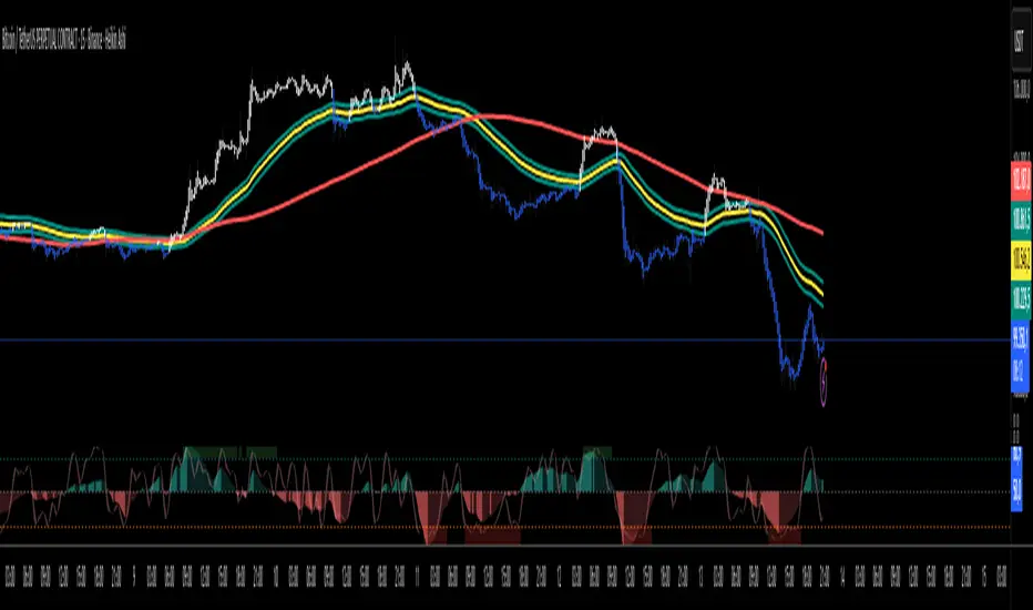
Range Oascilator + LessDivergences + MACD+StochRSIRange Oscillator + EMA Filter
Calculates a custom oscillator based on the highest high and lowest low over a chosen period.
Generates BUY signals when the oscillator crosses up from the oversold zone and price is above the EMA.
Generates SELL signals when the oscillator crosses down from the overbought zone and price is below the EMA.
MACD (3‑10‑16 EMA Settings)
Uses fast EMA = 3, slow EMA = 10, signal EMA = 16.
Detects bullish and bearish crossovers.
These crossovers only trigger a single unified buy/sell signal if they coincide with Stochastic RSI being in oversold (for buy) or overbought (for sell) zones.
Stochastic RSI
Standard calculation with %K and %D smoothing.
Defines oversold (<20) and overbought (>80) zones.
Used both for divergence detection and as a filter for MACD signals.
Divergence Detection
RSI Divergence: Price makes a lower low but RSI makes a higher low (bullish), or price makes a higher high but RSI makes a lower high (bearish).
MACD Histogram Divergence: Price makes a lower low but MACD histogram makes a higher low (bullish), or price makes a higher high but MACD histogram makes a lower high (bearish).
Stochastic RSI Divergence: Similar logic applied to %K line.
Divergences are flagged only once per pivot to avoid repetitive signals.
Visuals
EMA plotted on chart.
BUY/SELL signals shown as triangles above/below bars.
Divergences shown as labels (e.g., “RSI BullDiv”, “MACD BearDiv”).
Unified MACD+Stoch RSI signals shown in distinct colors (lime for buy, orange for sell).
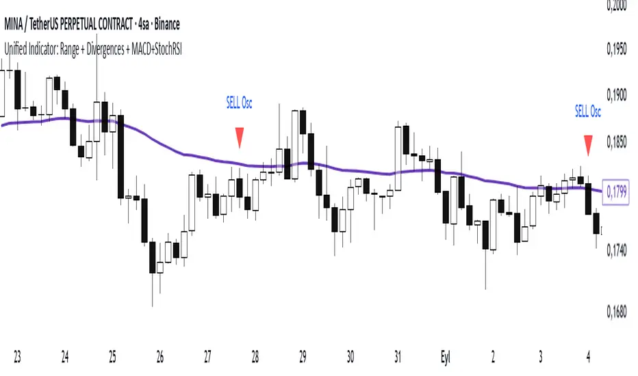
Trapper Absolute PriceActionThe Trapper Absolute PriceAction (TAPA) indicator is a custom, momentum-based oscillator designed to help traders visually read shifts in bullish and bearish price strength — with no reliance on volume or external data.
TAPA calculates and smooths both bullish and bearish momentum using multiple methods (RSI, Stochastic, or ADX) and compares their relative strength in real time. The result is a clean dual-line oscillator with color-coded histograms that highlight which side of the market currently has control.
It was built to give traders a sniper-level precision tool for detecting early momentum shifts before they appear clearly on price charts, allowing confirmation or invalidation of setups faster than with lagging indicators.
How It Works
Momentum Strength Calculation
The script measures directional price movement across the chosen mode (RSI, Stochastic, or ADX).
These values are smoothed twice using a selectable moving average type (WMA, EMA, SMA, ALMA, HMA, etc.).
Bullish & Bearish Curves
The green line represents smoothed bullish momentum (SmthBulls).
The orange/red line represents smoothed bearish momentum (SmthBears).
Histogram Strength Visualization
The distance between the two curves forms a color-coded histogram.
Green/Lime bars indicate growing bullish control, while Orange/Red bars show bearish dominance.
A gray neutral zone reflects indecision or range-bound conditions.
Signal Triggers
BUY 🐂 appears when the green line crosses up through the orange — signaling a bullish momentum flip.
SELL 🐻 appears when the green line crosses down through the orange — signaling bearish control.
Alerts can be enabled directly in TradingView through the BUY (🐂) or SELL (🐻) alert conditions for automated notifications or integrations.
How to Use
1. Confirm Early Momentum Shifts
When a crossover appears, check that the histogram color supports the move (green shades for bullish, red/orange for bearish).
Avoid signals when both lines are tangled and the histogram alternates gray, that usually indicates consolidation or low volatility.
2. Validate with Higher-Timeframe Structure
TAPA is most powerful when aligned with trend structure from higher timeframes.
Example: A bullish crossover on the 1-hour timeframe, while the daily TAPA shows the green line already rising, can confirm momentum alignment before entry.
3. Combine with Support/Resistance
Mark your key support and resistance zones (manual or using your “Trapper S&R PRO” indicator).
Look for a TAPA bullish crossover occurring at a major support zone, that’s often the start of a reversal move.
4. Multi-Mode Analysis
Experiment with “Indicator Method” in the inputs:
RSI Mode - smoother and responsive for swing trading.
Stochastic Mode - better for short-term entries and exits.
ADX Mode - captures trending momentum on strong breakouts.
Examples
Bullish Example:
Price forms a higher low on the chart while TAPA’s green line crosses up through orange with a lime/green histogram. That’s a strong early signal that momentum is reversing before price confirms on structure.
Bearish Example:
Price rallies into resistance, then TAPA shows a red histogram and a bearish cross (green dropping under orange). That’s typically a high-probability short signal once structure breaks.
What Makes TAPA Different
No Volume Dependency: Focuses purely on price behavior, not volume spikes or anomalies.
Multi-Mode Engine: Switch between RSI, Stochastic, or ADX-style momentum math instantly.
Customizable Visuals: Editable histogram color layers (weak/strong bull/bear, neutral) and line color control.
Sniper Labeling System: Clean, minimal BUY/SELL cues at each verified crossover.
Alert-Ready: Built-in conditions allow for TradingView alerts, webhooks, or bot automation.
Modernized Core: Rebuilt in Pine v6 with optimized performance and compliance to TradingView standards.
TAPA is designed to filter out the noise and show what truly drives a move — the shift in control between buyers and sellers.
Best Pairing Indicators
To get maximum clarity and confluence:
Trapper Support & Resistance PRO
Helps identify key zones where momentum flips from TAPA have the most impact. A bullish crossover at a defined support level often marks an early trend reversal.
Trapper Volume Trigger
While TAPA doesn’t use volume internally, pairing it with a volume-based trigger confirms that momentum shifts have institutional participation.
Simple Moving Averages (5, 20, or 50)
Overlay short and mid-term SMAs on your chart to confirm directional bias. A bullish TAPA cross that aligns with SMA-5 crossing above SMA-20 increases reliability.
Disclaimer
This indicator is provided for educational and analytical purposes only.
It does not constitute financial advice or a recommendation to buy or sell any security.
Always conduct your own due diligence and practice proper risk management before trading any strategy.
© 2025 RAMS-offthecharts | “Read • Analyze • Mark • Snipe.”
TAPA is part of the RAMS ecosystem of tactical market tools, designed for traders who focus on precision, discipline, and momentum awareness.
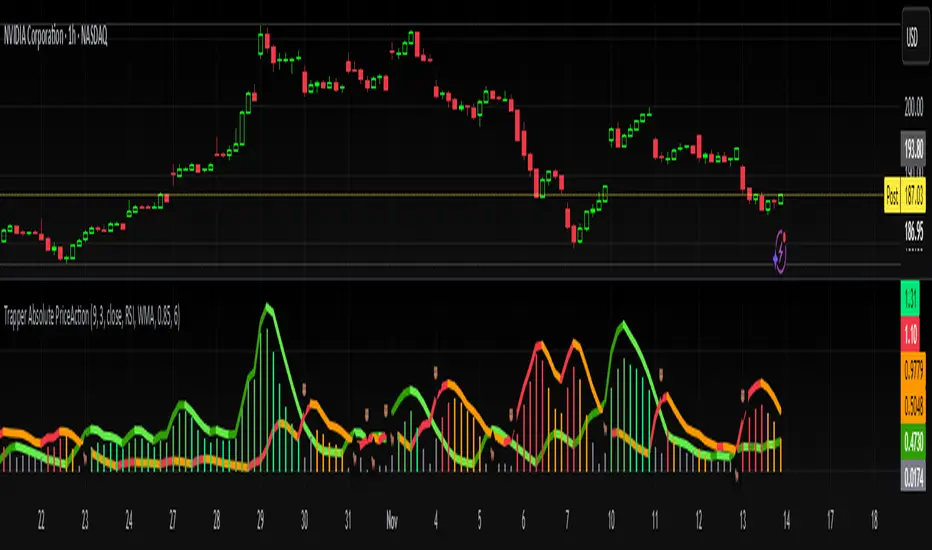
Range Oscillator Strategy + Stoch Confirm🔹 Short summary
This is a free, educational long-only strategy built on top of the public “Range Oscillator” by Zeiierman (used under CC BY-NC-SA 4.0), combined with a Stochastic timing filter, an EMA-based exit filter and an optional risk-management layer (SL/TP and R-multiple exits). It is NOT financial advice and it is NOT a magic money machine. It’s a structured framework to study how range-expansion + momentum + trend slope can be combined into one rule-based system, often with intentionally RARE trades.
────────────────────────
0. Legal / risk disclaimer
────────────────────────
• This script is FREE and public. I do not charge any fee for it.
• It is for EDUCATIONAL PURPOSES ONLY.
• It is NOT financial advice and does NOT guarantee profits.
• Backtest results can be very different from live results.
• Markets change over time; past performance is NOT indicative of future performance.
• You are fully responsible for your own trades and risk.
Please DO NOT use this script with money you cannot afford to lose. Always start in a demo / paper trading environment and make sure you understand what the logic does before you risk any capital.
────────────────────────
1. About default settings and risk (very important)
────────────────────────
The script is configured with the following defaults in the `strategy()` declaration:
• `initial_capital = 10000`
→ This is only an EXAMPLE account size.
• `default_qty_type = strategy.percent_of_equity`
• `default_qty_value = 100`
→ This means 100% of equity per trade in the default properties.
→ This is AGGRESSIVE and should be treated as a STRESS TEST of the logic, not as a realistic way to trade.
TradingView’s House Rules recommend risking only a small part of equity per trade (often 1–2%, max 5–10% in most cases). To align with these recommendations and to get more realistic backtest results, I STRONGLY RECOMMEND you to:
1. Open **Strategy Settings → Properties**.
2. Set:
• Order size: **Percent of equity**
• Order size (percent): e.g. **1–2%** per trade
3. Make sure **commission** and **slippage** match your own broker conditions.
• By default this script uses `commission_value = 0.1` (0.1%) and `slippage = 3`, which are reasonable example values for many crypto markets.
If you choose to run the strategy with 100% of equity per trade, please treat it ONLY as a stress-test of the logic. It is NOT a sustainable risk model for live trading.
────────────────────────
2. What this strategy tries to do (conceptual overview)
────────────────────────
This is a LONG-ONLY strategy designed to explore the combination of:
1. **Range Oscillator (Zeiierman-based)**
- Measures how far price has moved away from an adaptive mean.
- Uses an ATR-based range to normalize deviation.
- High positive oscillator values indicate strong price expansion away from the mean in a bullish direction.
2. **Stochastic as a timing filter**
- A classic Stochastic (%K and %D) is used.
- The logic requires %K to be below a user-defined level and then crossing above %D.
- This is intended to catch moments when momentum turns up again, rather than chasing every extreme.
3. **EMA Exit Filter (trend slope)**
- An EMA with configurable length (default 70) is calculated.
- The slope of the EMA is monitored: when the slope turns negative while in a long position, and the filter is enabled, it triggers an exit condition.
- This acts as a trend-protection exit: if the medium-term trend starts to weaken, the strategy exits even if the oscillator has not yet fully reverted.
4. **Optional risk-management layer**
- Percentage-based Stop Loss and Take Profit (SL/TP).
- Risk/Reward (R-multiple) exit based on the distance from entry to SL.
- Implemented as OCO orders that work *on top* of the logical exits.
The goal is not to create a “holy grail” system but to serve as a transparent, configurable framework for studying how these concepts behave together on different markets and timeframes.
────────────────────────
3. Components and how they work together
────────────────────────
(1) Range Oscillator (based on “Range Oscillator (Zeiierman)”)
• The script computes a weighted mean price and then measures how far price deviates from that mean.
• Deviation is normalized by an ATR-based range and expressed as an oscillator.
• When the oscillator is above the **entry threshold** (default 100), it signals a strong move away from the mean in the bullish direction.
• When it later drops below the **exit threshold** (default 30), it can trigger an exit (if enabled).
(2) Stochastic confirmation
• Classic Stochastic (%K and %D) is calculated.
• An entry requires:
- %K to be below a user-defined “Cross Level”, and
- then %K to cross above %D.
• This is a momentum confirmation: the strategy tries to enter when momentum turns up from a pullback rather than at any random point.
(3) EMA Exit Filter
• The EMA length is configurable via `emaLength` (default 70).
• The script monitors the EMA slope: it computes the relative change between the current EMA and the previous EMA.
• If the slope turns negative while the strategy holds a long position and the filter is enabled, it triggers an exit condition.
• This is meant to help protect profits or cut losses when the medium-term trend starts to roll over, even if the oscillator conditions are not (yet) signalling exit.
(4) Risk management (optional)
• Stop Loss (SL) and Take Profit (TP):
- Defined as percentages relative to average entry price.
- Both are disabled by default, but you can enable them in the Inputs.
• Risk/Reward Exit:
- Uses the distance from entry to SL to project a profit target at a configurable R-multiple.
- Also optional and disabled by default.
These exits are implemented as `strategy.exit()` OCO orders and can close trades independently of oscillator/EMA conditions if hit first.
────────────────────────
4. Entry & Exit logic (high level)
────────────────────────
A) Time filter
• You can choose a **Start Year** in the Inputs.
• Only candles between the selected start date and 31 Dec 2069 are used for backtesting (`timeCondition`).
• This prevents accidental use of tiny cherry-picked windows and makes tests more honest.
B) Entry condition (long-only)
A long entry is allowed when ALL the following are true:
1. `timeCondition` is true (inside the backtest window).
2. If `useOscEntry` is true:
- Range Oscillator value must be above `entryLevel`.
3. If `useStochEntry` is true:
- Stochastic condition (`stochCondition`) must be true:
- %K < `crossLevel`, then %K crosses above %D.
If these filters agree, the strategy calls `strategy.entry("Long", strategy.long)`.
C) Exit condition (logical exits)
A position can be closed when:
1. `timeCondition` is true AND a long position is open, AND
2. At least one of the following is true:
- If `useOscExit` is true: Oscillator is below `exitLevel`.
- If `useMagicExit` (EMA Exit Filter) is true: EMA slope is negative (`isDown = true`).
In that case, `strategy.close("Long")` is called.
D) Risk-management exits
While a position is open:
• If SL or TP is enabled:
- `strategy.exit("Long Risk", ...)` places an OCO stop/limit order based on the SL/TP percentages.
• If Risk/Reward exit is enabled:
- `strategy.exit("RR Exit", ...)` places an OCO order using a projected R-multiple (`rrMult`) of the SL distance.
These risk-based exits can trigger before the logical oscillator/EMA exits if price hits those levels.
────────────────────────
5. Recommended backtest configuration (to avoid misleading results)
────────────────────────
To align with TradingView House Rules and avoid misleading backtests:
1. **Initial capital**
- 10 000 (or any value you personally want to work with).
2. **Order size**
- Type: **Percent of equity**
- Size: **1–2%** per trade is a reasonable starting point.
- Avoid risking more than 5–10% per trade if you want results that could be sustainable in practice.
3. **Commission & slippage**
- Commission: around 0.1% if that matches your broker.
- Slippage: a few ticks (e.g. 3) to account for real fills.
4. **Timeframe & markets**
- Volatile symbols (e.g. crypto like BTCUSDT, or major indices).
- Timeframes: 1H / 4H / **1D (Daily)** are typical starting points.
- I strongly recommend trying the strategy on **different timeframes**, for example 1D, to see how the behaviour changes between intraday and higher timeframes.
5. **No “caution warning”**
- Make sure your chosen symbol + timeframe + settings do not trigger TradingView’s caution messages.
- If you see warnings (e.g. “too few trades”), adjust timeframe/symbol or the backtest period.
────────────────────────
5a. About low trade count and rare signals
────────────────────────
This strategy is intentionally designed to trade RARELY:
• It is **long-only**.
• It uses strict filters (Range Oscillator threshold + Stochastic confirmation + optional EMA Exit Filter).
• On higher timeframes (especially **1D / Daily**) this can result in a **low total number of trades**, sometimes WELL BELOW 100 trades over the whole backtest.
TradingView’s House Rules mention 100+ trades as a guideline for more robust statistics. In this specific case:
• The **low trade count is a conscious design choice**, not an attempt to cherry-pick a tiny, ultra-profitable window.
• The goal is to study a **small number of high-conviction long entries** on higher timeframes, not to generate frequent intraday signals.
• Because of the low trade count, results should NOT be interpreted as statistically strong or “proven” – they are only one sample of how this logic would have behaved on past data.
Please keep this in mind when you look at the equity curve and performance metrics. A beautiful curve with only a handful of trades is still just a small sample.
────────────────────────
6. How to use this strategy (step-by-step)
────────────────────────
1. Add the script to your chart.
2. Open the **Inputs** tab:
- Set the backtest start year.
- Decide whether to use Oscillator-based entry/exit, Stochastic confirmation, and EMA Exit Filter.
- Optionally enable SL, TP, and Risk/Reward exits.
3. Open the **Properties** tab:
- Set a realistic account size if you want.
- Set order size to a realistic % of equity (e.g. 1–2%).
- Confirm that commission and slippage are realistic for your broker.
4. Run the backtest:
- Look at Net Profit, Max Drawdown, number of trades, and equity curve.
- Remember that a low trade count means the statistics are not very strong.
5. Experiment:
- Tweak thresholds (`entryLevel`, `exitLevel`), Stochastic settings, EMA length, and risk params.
- See how the metrics and trade frequency change.
6. Forward-test:
- Before using any idea in live trading, forward-test on a demo account and observe behaviour in real time.
────────────────────────
7. Originality and usefulness (why this is more than a mashup)
────────────────────────
This script is not intended to be a random visual mashup of indicators. It is designed as a coherent, testable strategy with clear roles for each component:
• Range Oscillator:
- Handles mean vs. range-expansion states via an adaptive, ATR-normalized metric.
• Stochastic:
- Acts as a timing filter to avoid entering purely on extremes and instead waits for momentum to turn.
• EMA Exit Filter:
- Trend-slope-based safety net to exit when the medium-term direction changes against the position.
• Risk module:
- Provides practical, rule-based exits: SL, TP, and R-multiple exit, which are useful for structuring risk even if you modify the core logic.
It aims to give traders a ready-made **framework to study and modify**, not a black box or “signals” product.
────────────────────────
8. Limitations and good practices
────────────────────────
• No single strategy works on all markets or in all regimes.
• This script is long-only; it does not short the market.
• Performance can degrade when market structure changes.
• Overfitting (curve fitting) is a real risk if you endlessly tweak parameters to maximise historical profit.
Good practices:
- Test on multiple symbols and timeframes.
- Focus on stability and drawdown, not only on how high the profit line goes.
- View this as a learning tool and a basis for your own research.
────────────────────────
9. Licensing and credits
────────────────────────
• Core oscillator idea & base code:
- “Range Oscillator (Zeiierman)”
- © Zeiierman, licensed under CC BY-NC-SA 4.0.
• Strategy logic, Stochastic confirmation, EMA Exit Filter, and risk-management layer:
- Modifications by jokiniemi.
Please respect both the original license and TradingView House Rules if you fork or republish any part of this script.
────────────────────────
10. No payments / no vendor pitch
────────────────────────
• This script is completely FREE to use on TradingView.
• There is no paid subscription, no external payment link, and no private signals group attached to it.
• If you have questions, please use TradingView’s comment system or private messages instead of expecting financial advice.
Use this script as a tool to learn, experiment, and build your own understanding of markets.
────────────────────────
11. Example backtest settings used in screenshots
────────────────────────
To avoid any confusion about how the results shown in screenshots were produced, here is one concrete example configuration:
• Symbol: BTCUSDT (or similar major BTC pair)
• Timeframe: 1D (Daily)
• Backtest period: from 2018 to the most recent data
• Initial capital: 10 000
• Order size type: Percent of equity
• Order size: 2% per trade
• Commission: 0.1%
• Slippage: 3 ticks
• Risk settings: Stop Loss and Take Profit disabled by default, Risk/Reward exit disabled by default
• Filters: Range Oscillator entry/exit enabled, Stochastic confirmation enabled, EMA Exit Filter enabled
If you change any of these settings (symbol, timeframe, risk per trade, commission, slippage, filters, etc.), your results will look different. Please always adapt the configuration to your own risk tolerance, market, and trading style.