إدارة المحافظ الاستثمارية

BTC Fear & Greed Incremental StrategyIMPORTANT: READ SETUP GUIDE BELOW OR IT WON'T WORK
# BTC Fear & Greed Incremental Strategy — TradeMaster AI (Pure BTC Stack)
## Strategy Overview
This advanced Bitcoin accumulation strategy is designed for long-term hodlers who want to systematically take profits during greed cycles and accumulate during fear periods, while preserving their core BTC position. Unlike traditional strategies that start with cash, this approach begins with a specified BTC allocation, making it perfect for existing Bitcoin holders who want to optimize their stack management.
## Key Features
### 🎯 **Pure BTC Stack Mode**
- Start with any amount of BTC (configurable)
- Strategy manages your existing stack, not new purchases
- Perfect for hodlers who want to optimize without timing markets
### 📊 **Fear & Greed Integration**
- Uses market sentiment data to drive buy/sell decisions
- Configurable thresholds for greed (selling) and fear (buying) triggers
- Automatic validation to ensure proper 0-100 scale data source
### 🐂 **Bull Year Optimization**
- Smart quarterly selling during bull market years (2017, 2021, 2025)
- Q1: 1% sells, Q2: 2% sells, Q3/Q4: 5% sells (configurable)
- **NO SELLING** during non-bull years - pure accumulation mode
- Preserves BTC during early bull phases, maximizes profits at peaks
### 🐻 **Bear Market Intelligence**
- Multi-regime detection: Bull, Early Bear, Deep Bear, Early Bull
- Different buying strategies based on market conditions
- Enhanced buying during deep bear markets with configurable multipliers
- Visual regime backgrounds for easy market condition identification
### 🛡️ **Risk Management**
- Minimum BTC allocation floor (prevents selling entire stack)
- Configurable position sizing for all trades
- Multiple safety checks and validation
### 📈 **Advanced Visualization**
- Clean 0-100 scale with 2 decimal precision
- Three main indicators: BTC Allocation %, Fear & Greed Index, BTC Holdings
- Real-time portfolio tracking with cash position display
- Enhanced info table showing all key metrics
## How to Use
### **Step 1: Setup**
1. Add the strategy to your BTC/USD chart (daily timeframe recommended)
2. **CRITICAL**: In settings, change the "Fear & Greed Source" from "close" to a proper 0-100 Fear & Greed indicator
---------------
I recommend Crypto Fear & Greed Index by TIA_Technology indicator
When selecting source with this indicator, look for "Crypto Fear and Greed Index:Index"
---------------
3. Set your "Starting BTC Quantity" to match your actual holdings
4. Configure your preferred "Start Date" (when you want the strategy to begin)
### **Step 2: Configure Bull Year Logic**
- Enable "Bull Year Logic" (default: enabled)
- Adjust quarterly sell percentages:
- Q1 (Jan-Mar): 1% (conservative early bull)
- Q2 (Apr-Jun): 2% (moderate mid bull)
- Q3/Q4 (Jul-Dec): 5% (aggressive peak targeting)
- Add future bull years to the list as needed
### **Step 3: Fine-tune Thresholds**
- **Greed Threshold**: 80 (sell when F&G > 80)
- **Fear Threshold**: 20 (buy when F&G < 20 in bull markets)
- **Deep Bear Fear Threshold**: 25 (enhanced buying in bear markets)
- Adjust based on your risk tolerance
### **Step 4: Risk Management**
- Set "Minimum BTC Allocation %" (default 20%) - prevents selling entire stack
- Configure sell/buy percentages based on your position size
- Enable bear market filters for enhanced timing
### **Step 5: Monitor Performance**
- **Orange Line**: Your BTC allocation percentage (target: fluctuate between 20-100%)
- **Blue Line**: Actual BTC holdings (should preserve core position)
- **Pink Line**: Fear & Greed Index (drives all decisions)
- **Table**: Real-time portfolio metrics including cash position
## Reading the Indicators
### **BTC Allocation Percentage (Orange Line)**
- **100%**: All portfolio in BTC, no cash available for buying
- **80%**: 80% BTC, 20% cash ready for fear buying
- **20%**: Minimum allocation, maximum cash position
### **Trading Signals**
- **Green Buy Signals**: Appear during fear periods with available cash
- **Red Sell Signals**: Appear during greed periods in bull years only
- **No Signals**: Either allocation limits reached or non-bull year
## Strategy Logic
### **Bull Years (2017, 2021, 2025)**
- Q1: Conservative 1% sells (preserve stack for later)
- Q2: Moderate 2% sells (gradual profit taking)
- Q3/Q4: Aggressive 5% sells (peak targeting)
- Fear buying active (accumulate on dips)
### **Non-Bull Years**
- **Zero selling** - pure accumulation mode
- Enhanced fear buying during bear markets
- Focus on rebuilding stack for next bull cycle
## Important Notes
- **This is not financial advice** - backtest thoroughly before use
- Designed for **long-term holders** (4+ year cycles)
- **Requires proper Fear & Greed data source** - validate in settings
- Best used on **daily timeframe** for major trend following
- **Cash calculations**: Use allocation % and BTC holdings to calculate available cash: `Cash = (Total Portfolio × (1 - Allocation%/100))`
## Risk Disclaimer
This strategy involves active trading and position management. Past performance does not guarantee future results. Always do your own research and never invest more than you can afford to lose. The strategy is designed for educational purposes and long-term Bitcoin accumulation thesis.
---
*Developed by Sol_Crypto for the Bitcoin community. Happy stacking! 🚀*

Oracle Protocol — Arch Public (Testing Clone) Oracle Protocol — Arch Public Series (testing clone)
This model implements the Arch Public Oracle structure: a systematic accumulation-and-distribution engine built around a dynamic Accumulation Cost Base (ACB), strict profit-gate exit logic, and a capital-bounded flywheel reinvestment system.
It is designed for transparent execution, deterministic behaviour, and rule-based position management.
Core Function Set
1. Accumulation Framework (ACB-Driven)
The accumulation engine evaluates market movement against defined entry conditions, including:
Percentage-based entry-drop triggers
Optional buy-below-ACB mode
Capital-gated entries tied to available ledger balance
Fixed-dollar and min-dollar entry rules (as seen in Arch public materials)
Automated sizing through flywheel capital
Range-bounded ledger for controlled backtesting input
Each qualifying buy updates the live ACB, maintains the internal ledger, and forms the next reference point for exit evaluation.
No forecasting mechanisms are included.
2. Profit-Gate Exit System
Exits are governed by the standard Arch public approach:
A sealed ACB reference for threshold evaluation
Optional live-ACB visibility
Profit-gate triggers defined per asset class
Candle-confirmation integration (“ProfitGate + Candle” mode)
Distribution only when the smallest active threshold is met
This provides a consistent cadence with published Arch diagrams and PDFs.
3. Once-Per-Rally Governance
After a distribution, the algorithm locks until price retraces below the most recent accumulation base.
Only after re-arming can the next profit gate activate.
This prevents over-frequency selling and aligns with the public-domain Oracle behaviour.
4. Quiet-Bars & Threshold Cluster Control
A volatility-stabilisation layer prevents multiple exits from micro-fluctuations or transient spikes.
This ensures clean execution during fast markets and high volatility.
5. Flywheel Reinvestment
Distribution proceeds automatically return to the capital pool where permitted, creating a closed system of:
Entry sizing
Exit proceeds
Ledger-managed capital state
All sizing respects capital boundaries and does not breach dollar floors or overrides.
6. Automation Hooks and Integration
The script exposes:
3Commas-compatible JSON sizing
Entry/exit signalling via alertcondition()
Deterministic event reporting suitable for external automation
This allows consistent deployment across automated execution environments.
7. Visual Tooling
Optional displays include:
Live ACB line
Exit-guide markers
Capital, state, and ledger panels
Realized/unrealized outcome tracking based on internal logic only
Visual components do not influence execution rules.
Operating Notes
This model is rule-based, deterministic, and non-predictive.
It executes only according to the explicit thresholds, capital limits, and state transitions defined within the script.
No discretionary or forward-looking logic is included.

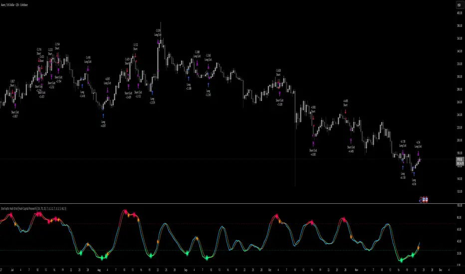
Stochastic Hash Strat [Hash Capital Research]# Stochastic Hash Strategy by Hash Capital Research
## 🎯 What Is This Strategy?
The **Stochastic Slow Strategy** is a momentum-based trading system that identifies oversold and overbought market conditions to capture mean-reversion opportunities. Think of it as a "buy low, sell high" approach with smart mathematical filters that remove emotion from your trading decisions.
Unlike fast-moving indicators that generate excessive noise, this strategy uses **smoothed stochastic oscillators** to identify only the highest-probability setups when momentum truly shifts.
---
## 💡 Why This Strategy Works
Most traders fail because they:
- **Chase prices** after big moves (buying high, selling low)
- **Overtrade** in choppy, directionless markets
- **Exit too early** or hold losses too long
This strategy solves all three problems:
1. **Entry Discipline**: Only trades when the stochastic oscillator crosses in extreme zones (oversold for longs, overbought for shorts)
2. **Cooldown Filter**: Prevents revenge trading by forcing a waiting period after each trade
3. **Fixed Risk/Reward**: Pre-defined stop-loss and take-profit levels ensure consistent risk management
**The Math Behind It**: The stochastic oscillator measures where the current price sits relative to its recent high-low range. When it's below 25, the market is oversold (time to buy). When above 70, it's overbought (time to sell). The crossover with its moving average confirms momentum is shifting.
---
## 📊 Best Markets & Timeframes
### ⭐ OPTIMAL PERFORMANCE:
**Crude Oil (WTI) - 12H Timeframe**
- **Why it works**: Oil markets have predictable volatility patterns and respect technical levels
**AAVE/USD - 4H to 12H Timeframe**
- **Why it works**: DeFi tokens exhibit strong momentum cycles with clear extremes
### ✅ Also Works Well On:
- **BTC/USD** (12H, Daily) - Lower frequency but high win rate
- **ETH/USD** (8H, 12H) - Balanced volatility and liquidity
- **Gold (XAU/USD)** (Daily) - Classic mean-reversion asset
- **EUR/USD** (4H, 8H) - Lower volatility, requires patience
### ❌ Avoid Using On:
- Timeframes below 4H (too much noise)
- Low-liquidity altcoins (wide spreads kill performance)
- Strongly trending markets without pullbacks (Bitcoin in 2021)
- News-driven instruments during major events
---
## 🎛️ Understanding The Settings
### Core Stochastic Parameters
**Stochastic Length (Default: 16)**
- Controls the lookback period for price comparison
- Lower = faster reactions, more signals (10-14 for volatile markets)
- Higher = smoother signals, fewer trades (16-21 for stable markets)
- **Pro tip**: Use 10 for crypto 4H, 16 for commodities 12H
**Overbought Level (Default: 70)**
- Threshold for short entries
- Lower values (65-70) = more trades, earlier entries
- Higher values (75-80) = fewer but higher-conviction trades
- **Sweet spot**: 70 works for most assets
**Oversold Level (Default: 25)**
- Threshold for long entries
- Higher values (25-30) = more trades, earlier entries
- Lower values (15-20) = fewer but stronger bounce setups
- **Sweet spot**: 20-25 depending on market conditions
**Smooth K & Smooth D (Default: 7 & 3)**
- Additional smoothing to filter out whipsaws
- K=7 makes the indicator slower and more reliable
- D=3 is the signal line that confirms the trend
- **Don't change these unless you know what you're doing**
---
### Risk Management
**Stop Loss % (Default: 2.2%)**
- Automatically exits losing trades
- Should be 1.5x to 2x your average market volatility
- Too tight = death by a thousand cuts
- Too wide = uncontrolled losses
- **Calibration**: Check ATR indicator and set SL slightly above it
**Take Profit % (Default: 7%)**
- Automatically exits winning trades
- Should be 2.5x to 3x your stop loss (reward-to-risk ratio)
- This default gives 7% / 2.2% = 3.18:1 R:R
- **The golden rule**: Never have R:R below 2:1
---
### Trade Filters
**Bar Cooldown Filter (Default: ON, 3 bars)**
- **What it does**: Forces you to wait X bars after closing a trade before entering a new one
- **Why it matters**: Prevents emotional revenge trading and overtrading in choppy markets
- **Settings guide**:
- 3 bars = Standard (good for most cases)
- 5-7 bars = Conservative (oil, slow-moving assets)
- 1-2 bars = Aggressive (only for experienced traders)
**Exit on Opposite Extreme (Default: ON)**
- Closes your long when stochastic hits overbought (and vice versa)
- Acts as an early profit-taking mechanism
- **Leave this ON** unless you're testing other exit strategies
**Divergence Filter (Default: OFF)**
- Looks for price/momentum divergences for additional confirmation
- **When to enable**: Trending markets where you want fewer but higher-quality trades
- **Keep OFF for**: Mean-reverting markets (oil, forex, most of the time)
---
## 🚀 Quick Start Guide
### Step 1: Set Up in TradingView
1. Open TradingView and navigate to your chart
2. Click "Pine Editor" at the bottom
3. Copy and paste the strategy code
4. Click "Add to Chart"
5. The strategy will appear in a separate pane below your price chart
### Step 2: Choose Your Market
**If you're trading Crude Oil:**
- Timeframe: 12H
- Keep all default settings
- Watch for signals during London/NY overlap (8am-11am EST)
**If you're trading AAVE or crypto:**
- Timeframe: 4H or 12H
- Consider these adjustments:
- Stochastic Length: 10-14 (faster)
- Oversold: 20 (more aggressive)
- Take Profit: 8-10% (higher targets)
### Step 3: Wait for Your First Signal
**LONG Entry** (Green circle appears):
- Stochastic crosses up below oversold level (25)
- Price likely near recent lows
- System places limit order at take profit and stop loss
**SHORT Entry** (Red circle appears):
- Stochastic crosses down above overbought level (70)
- Price likely near recent highs
- System places limit order at take profit and stop loss
**EXIT** (Orange circle):
- Position closes either at stop, target, or opposite extreme
- Cooldown period begins
### Step 4: Let It Run
The biggest mistake? **Interfering with the system.**
- Don't close trades early because you're scared
- Don't skip signals because you "have a feeling"
- Don't increase position size after a big win
- Don't revenge trade after a loss
**Follow the system or don't use it at all.**
---
### Important Risks:
1. **Drawdown Pain**: You WILL experience losing streaks of 5-7 trades. This is mathematically normal.
2. **Whipsaw Markets**: Choppy, range-bound conditions can trigger multiple small losses.
3. **Gap Risk**: Overnight gaps can cause your actual fill to be worse than the stop loss.
4. **Slippage**: Real execution prices differ from backtested prices (factor in 0.1-0.2% slippage).
---
## 🔧 Optimization Guide
### When to Adjust Settings:
**Market Volatility Increased?**
- Widen stop loss by 0.5-1%
- Increase take profit proportionally
- Consider increasing cooldown to 5-7 bars
**Getting Too Few Signals?**
- Decrease stochastic length to 10-12
- Increase oversold to 30, decrease overbought to 65
- Reduce cooldown to 2 bars
**Getting Too Many Losses?**
- Increase stochastic length to 18-21 (slower, smoother)
- Enable divergence filter
- Increase cooldown to 5+ bars
- Verify you're on the right timeframe
### A/B Testing Method:
1. **Run default settings for 50 trades** on your chosen market
2. Document: Win rate, profit factor, max drawdown, emotional tolerance
3. **Change ONE variable** (e.g., oversold from 25 to 20)
4. Run another 50 trades
5. Compare results
6. Keep the better version
**Never change multiple settings at once** or you won't know what worked.
---
## 📚 Educational Resources
### Key Concepts to Learn:
**Stochastic Oscillator**
- Developed by George Lane in the 1950s
- Measures momentum by comparing closing price to price range
- Formula: %K = (Close - Low) / (High - Low) × 100
- Similar to RSI but more sensitive to price movements
**Mean Reversion vs. Trend Following**
- This is a **mean reversion** strategy (price returns to average)
- Works best in ranging markets with defined support/resistance
- Fails in strong trending markets (2017 Bitcoin, 2020 Tech stocks)
- Complement with trend filters for better results
**Risk:Reward Ratio**
- The cornerstone of profitable trading
- Winning 40% of trades with 3:1 R:R = profitable
- Winning 60% of trades with 1:1 R:R = breakeven (after fees)
- **This strategy aims for 45% win rate with 2.5-3:1 R:R**
### Recommended Reading:
- *"Trading Systems and Methods"* by Perry Kaufman (Chapter on Oscillators)
- *"Mean Reversion Trading Systems"* by Howard Bandy
- *"The New Trading for a Living"* by Dr. Alexander Elder
---
## 🛠️ Troubleshooting
### "I'm not seeing any signals!"
**Check:**
- Is your timeframe 4H or higher?
- Is the stochastic actually reaching extreme levels (check if your asset is stuck in middle range)?
- Is cooldown still active from a previous trade?
- Are you on a low-liquidity pair?
**Solution**: Switch to a more volatile asset or lower the overbought/oversold thresholds.
---
### "The strategy keeps losing money!"
**Check:**
- What's your win rate? (Below 35% is concerning)
- What's your profit factor? (Below 0.8 means serious issues)
- Are you trading during major news events?
- Is the market in a strong trend?
**Solution**:
1. Verify you're using recommended markets/timeframes
2. Increase cooldown period to avoid choppy markets
3. Reduce position size to 5% while you diagnose
4. Consider switching to daily timeframe for less noise
---
### "My stop losses keep getting hit!"
**Check:**
- Is your stop loss tighter than the average ATR?
- Are you trading during high-volatility sessions?
- Is slippage eating into your buffer?
**Solution**:
1. Calculate the 14-period ATR
2. Set stop loss to 1.5x the ATR value
3. Avoid trading right after market open or major news
4. Factor in 0.2% slippage for crypto, 0.1% for oil
---
## 💪 Pro Tips from the Trenches
### Psychological Discipline
**The Three Deadly Sins:**
1. **Skipping signals** - "This one doesn't feel right"
2. **Early exits** - "I'll just take profit here to be safe"
3. **Revenge trading** - "I need to make back that loss NOW"
**The Solution:** Treat your strategy like a business system. Would McDonald's skip making fries because the cashier "doesn't feel like it today"? No. Systems work because of consistency.
---
### Position Management
**Scaling In/Out** (Advanced)
- Enter 50% position at signal
- Add 50% if stochastic reaches 10 (oversold) or 90 (overbought)
- Exit 50% at 1.5x take profit, let the rest run
**This is NOT for beginners.** Master the basic system first.
---
### Market Awareness
**Oil Traders:**
- OPEC meetings = volatility spikes (avoid or widen stops)
- US inventory reports (Wed 10:30am EST) = avoid trading 2 hours before/after
- Summer driving season = different patterns than winter
**Crypto Traders:**
- Monday-Tuesday = typically lower volatility (fewer signals)
- Thursday-Sunday = higher volatility (more signals)
- Avoid trading during exchange maintenance windows
---
## ⚖️ Legal Disclaimer
This trading strategy is provided for **educational purposes only**.
- Past performance does not guarantee future results
- Trading involves substantial risk of loss
- Only trade with capital you can afford to lose
- No one associated with this strategy is a licensed financial advisor
- You are solely responsible for your trading decisions
**By using this strategy, you acknowledge that you understand and accept these risks.**
---
## 🙏 Acknowledgments
Strategy development inspired by:
- George Lane's original Stochastic Oscillator work
- Modern quantitative trading research
- Community feedback from hundreds of backtests
Built with ❤️ for retail traders who want systematic, disciplined approaches to the markets.
---
**Good luck, stay disciplined, and trade the system, not your emotions.**
Hash Supertrend [Hash Capital Research]Hash Supertrend Strategy by Hash Capital Research
Overview
Hash Supertrend is a professional-grade trend-following strategy that combines the proven Supertrend indicator with institutional visual design and flexible time filtering.
The strategy uses ATR-based volatility bands to identify trend direction and executes position reversals when the trend flips.This implementation features a distinctive fluorescent color system with customizable glow effects, making trend changes immediately visible while maintaining the clean, professional aesthetic expected in quantitative trading environments.
Entry Signals:
Long Entry: Price crosses above the Supertrend line (trend flips bullish)
Short Entry: Price crosses below the Supertrend line (trend flips bearish)
Controls the lookback period for volatility calculation
Lower values (7-10): More sensitive to price changes, generates more signals
Higher values (12-14): Smoother response, fewer signals but potentially delayed entries
Recommended range: 7-14 depending on market volatility
Factor (Default: 3.0)
Restricts trading to specific hours
Useful for avoiding low-liquidity sessions, overnight gaps, or known choppy periods
When disabled, strategy trades 24/7
Start Hour (Default: 9) & Start Minute (Default: 30)
Define when the trading session begins
Uses exchange timezone in 24-hour format
Example: 9:30 = 9:30 AM
End Hour (Default: 16) & End Minute (Default: 0)
Controls the vibrancy of the fluorescent color system
1-3: Subtle, muted colors
4-6: Balanced, moderate saturation
7-10: Bright, highly saturated fluorescent appearance
Affects both the Supertrend line and trend zones
Glow Effect (Default: On)
Adds luminous halo around the Supertrend line
Creates a multi-layered visual with depth
Particularly effective during strong trends
Glow Intensity (Default: 5.0)
Displays tiny fluorescent dots at entry points
Green dot below bar: Long entry
Red dot above bar: Short entry
Provides clear visual confirmation of executed trades
Show Trend Zone (Default: On)
Strong trending markets (2020-style bull runs, sustained bear markets)
Markets with clear directional bias
Instruments with consistent volatility patterns
Timeframes: 15m to Daily (optimal on 1H-4H)
Challenging Conditions:
Choppy, range-bound markets
Low volatility consolidation periods
Highly news-driven instruments with frequent gaps
Very low timeframes (1m-5m) prone to noise
Recommended AssetsCryptocurrency:

ATH대비 지정하락률에 도착 시 매수 - 장기홀딩 선물 전략(ATH Drawdown Re-Buy Long Only)본 스크립트는 과거 하락 데이터를 이용하여, 정해진 하락 %가 발생하는 경우 자기 자본의 정해진 %만큼을 진입하게 설계되어진 스트레티지입니다.
레버리지를 사용할 수 있으며 기본적으로 셋팅해둔 값이 내장되어있습니다.(자유롭게 바꿔서 쓰시면 됩니다.) 추가적으로 2번의 진입 외에도 다른 진입 기준, 진입 %를 설정하실 수 있으며 - ChatGPT에게 요청하면 수정해줄 것입니다.
실제 사용용도로는 KillSwitch 기능을 꺼주세요. 바 돋보기 기능을 켜주세요.
ATH Drawdown Re-Buy Long Only 전략 설명
1. 전략 개요
ATH Drawdown Re-Buy Long Only 전략은 자산의 역대 최고가(ATH, All-Time High)를 기준으로 한 하락폭(드로우다운)을 활용하여,
특정 구간마다 단계적으로 롱 포지션을 구축하는 자동 재매수(Long Only) 전략입니다.
본 전략은 다음과 같은 목적을 가지고 설계되었습니다.
급격한 조정 구간에서 체계적인 분할 매수 및 레버리지 활용
ATH를 기준으로 한 명확한 진입 규칙 제공
실시간으로
평단가
레버리지
청산가 추정
계좌 MDD
수익률
등을 시각적으로 제공하여 리스크와 포지션 상태를 직관적으로 확인할 수 있도록 지원
※ 본 전략은 교육·연구·백테스트 용도로 제공되며,
어떠한 형태의 투자 권유 또는 수익을 보장하지 않습니다.
2. 전략의 핵심 개념
2-1. ATH(역대 최고가) 기준 드로우다운
전략은 차트 상에서 항상 가장 높은 고가(High)를 ATH로 기록합니다.
새로운 고점이 형성될 때마다 ATH를 갱신하고, 해당 ATH를 기준으로 다음을 계산합니다.
현재 바의 저가(Low)가 ATH에서 몇 % 하락했는지
현재 바의 종가(Close)가 ATH에서 몇 % 하락했는지
그리고 사전에 설정한 두 개의 드로우다운 구간에서 매수를 수행합니다.
1차 진입 구간: ATH 대비 X% 하락 시
2차 진입 구간: ATH 대비 Y% 하락 시
각 구간은 ATH가 새로 갱신될 때마다 한 번씩만 작동하며,
새로운 ATH가 생성되면 다시 “1차 / 2차 진입 가능 상태”로 초기화됩니다.
2-2. 첫 포지션 100% / 300% 특수 규칙
이 전략의 중요한 특징은 **“첫 포지션 진입 시의 예외 규칙”**입니다.
전략이 현재 어떠한 포지션도 들고 있지 않은 상태에서
최초로 롱 포지션을 진입하는 시점(첫 포지션)에 대해:
기본적으로는 **자산의 100%**를 기준으로 포지션을 구축하지만,
만약 그 순간의 가격이 ATH 대비 설정값 이상(예: 약 –72.5% 이상 하락한 상황) 이라면
→ 자산의 300% 규모로 첫 포지션을 진입하도록 설계되어 있습니다.
이 규칙은 다음과 같이 동작합니다.
첫 진입이 1차 드로우다운 구간에서 발생하든,
첫 진입이 2차 드로우다운 구간에서 발생하든,
현재 하락폭이 설정된 기준 이상(예: –72.5% 이상) 이라면
→ “이 정도 하락이면 첫 진입부터 더 공격적으로 들어간다”는 의미로 300% 규모로 진입
그 이하의 하락폭이라면
→ 첫 진입은 100% 규모로 제한
즉, 전략은 다음 두 가지 모드로 동작합니다.
일반적인 상황의 첫 진입: 자산의 100%
심각한 드로우다운 구간에서의 첫 진입: 자산의 300%
이 특수 규칙은 깊은 하락에서는 공격적으로, 평소에는 상대적으로 보수적으로 진입하도록 설계된 것입니다.
3. 전략 동작 구조
3-1. 매수 조건
차트 상 High 기준으로 ATH를 추적합니다.
각 바마다 해당 ATH에서의 하락률을 계산합니다.
사용자가 설정한 두 개의 드로우다운 구간(예시):
1차 구간: 예를 들어 ATH – 50%
2차 구간: 예를 들어 ATH – 72.5%
각 구간에 대해 다음과 같은 조건을 확인합니다.
“이번 ATH 구간에서 아직 해당 구간 매수를 한 적이 없는 상태”이고,
현재 바의 저가(Low)가 해당 구간 가격 이하를 찍는 순간
→ 해당 바에서 매수 조건 충족으로 간주
실제 주문은:
해당 구간 가격에 맞춰 롱 포지션 진입(리밋/시장가 기반 시뮬레이션) 으로 처리됩니다.
3-2. ATH 갱신과 진입 기회 리셋
차트 상에서 새로운 고점(High)이 기존 ATH를 넘어서는 순간,
ATH가 갱신되고,
1차 / 2차 진입 여부를 나타내는 내부 플래그가 초기화됩니다.
이를 통해, 시장이 새로운 고점을 돌파해 나갈 때마다,
해당 구간에서 다시 한 번씩 1차·2차 드로우다운 진입 기회를 갖게 됩니다.
4. 포지션 사이징 및 레버리지
4-1. 계좌 자산(Equity) 기준 포지션 크기 결정
전략은 현재 계좌 자산을 다음과 같이 정의하여 사용합니다.
현재 자산 = 초기 자본 + 실현 손익 + 미실현 손익
각 진입 구간에서의 포지션 가치는 다음과 같이 결정됩니다.
1차 진입 구간:
“자산의 몇 %를 사용할지”를 설정값으로 입력
설정된 퍼센트를 계좌 자산에 곱한 뒤,
다시 전략 내 레버리지 배수(Leverage) 를 곱하여 실제 포지션 가치를 계산
2차 진입 구간:
동일한 방식으로, 독립된 퍼센트 설정값을 사용
즉, 포지션 가치는 다음과 같이 계산됩니다.
포지션 가치 = 현재 자산 × (해당 구간 설정 % / 100) × 레버리지 배수
그리고 이를 해당 구간의 진입 가격으로 나누어 실제 수량(토큰 단위) 를 산출합니다.
4-2. 첫 포지션의 예외 처리 (100% / 300%)
첫 포지션에 대해서는 위의 일반적인 퍼센트 설정 대신,
다음과 같은 고정 비율이 사용됩니다.
기본: 자산의 100% 규모로 첫 포지션 진입
단, 진입 시점의 ATH 대비 하락률이 설정값 이상(예: –72.5% 이상) 일 경우
→ 자산의 300% 규모로 첫 포지션 진입
이때 역시 다음 공식을 사용합니다.
포지션 가치 = 현재 자산 × (100% 또는 300%) × 레버리지
그리고 이를 가격으로 나누어 실제 진입 수량을 계산합니다.
이 규칙은:
첫 진입이 1차 구간이든 2차 구간이든 동일하게 적용되며,
“충분히 깊은 하락 구간에서는 첫 진입부터 더 크게,
평소에는 비교적 보수적으로” 라는 운용 철학을 반영합니다.
4-3. 실레버리지(Real Leverage)의 추적
전략은 각 바 단위로 다음을 추적합니다.
바가 시작할 때의 기존 포지션 크기
해당 바에서 새로 진입한 수량
이를 바탕으로, 진입이 발생한 시점에 다음을 계산합니다.
실제 레버리지 = (포지션 가치 / 현재 자산)
그리고 차트 상에 예를 들어:
Lev 2.53x 와 같은 형식의 레이블로 표시합니다.
이를 통해, 매수 시점마다 실제 계좌 레버리지가 어느 정도였는지를 직관적으로 확인할 수 있습니다.
5. 시각화 및 모니터링 요소
5-1. 차트 상 시각 요소
전략은 차트 위에 다음과 같은 정보를 직접 표시합니다.
ATH 라인
High 기준으로 계산된 역대 최고가를 주황색 선으로 표시
평단가(평균 진입가) 라인
현재 보유 포지션이 있을 때,
해당 포지션의 평균 진입가를 노란색 선으로 표시
추정 청산가(고정형 청산가) 라인
포지션 수량이 변화하는 시점을 감지하여,
당시의 평단가와 실제 레버리지를 이용해 근사적인 청산가를 계산
이를 빨간색 선으로 차트에 고정 표시
포지션이 없거나 레버리지가 1배 이하인 경우에는 청산가 라인을 제거
매수 마커 및 레이블
1차/2차 매수 조건이 충족될 때마다 해당 지점에 매수 마커를 표시
"Buy XX% @ 가격", "Lev XXx" 형태의 라벨로
진입 비율과 당시 레버리지를 함께 시각화
레이블의 위치는 설정에서 선택 가능:
바 아래 (Below Bar)
바 위 (Above Bar)
실제 가격 위치 (At Price)
5-2. 우측 상단 정보 테이블
차트 우측 상단에는 현재 계좌·포지션 상태를 요약한 정보 테이블이 표시됩니다.
대표적으로 다음 항목들이 포함됩니다.
Pos Qty (Token)
현재 보유 중인 포지션 수량(토큰 기준, 절대값 기준)
Pos Value (USDT)
현재 포지션의 시장 가치 (수량 × 현재 가격)
Leverage (Now)
현재 실레버리지 (포지션 가치 / 현재 자산)
DD from ATH (%)
현재 가격 기준, 최근 ATH에서의 하락률(%)
Avg Entry
현재 포지션의 평균 진입 가격
PnL (%)
현재 포지션 기준 미실현 손익률(%)
Max DD (Equity %)
전략 전체 기간 동안 기록된 계좌 기준 최대 손실(MDD, Max Drawdown)
Last Entry Price
가장 최근에 포지션을 추가로 진입한 직후의 평균 진입 가격
Last Entry Lev
위 “Last Entry Price” 시점에서의 실레버리지
Liq Price (Fixed)
위에서 설명한 고정형 추정 청산가
Return from Start (%)
전략 시작 시점(초기 자본) 대비 현재 계좌 자산의 총 수익률(%)
이 테이블을 통해 사용자는:
현재 계좌와 포지션의 상태
리스크 수준
누적 성과
를 직관적으로 파악할 수 있습니다.
6. 시간 필터 및 라벨 옵션
6-1. 전략 동작 기간 설정
전략은 옵션으로 특정 기간에만 전략을 동작시키는 시간 필터를 제공합니다.
“Use Date Range” 옵션을 활성화하면:
시작 시각과 종료 시각을 지정하여
해당 구간에 한해서만 매매가 발생하도록 제한
옵션을 비활성화하면:
전략은 전체 차트 구간에서 자유롭게 동작
6-2. 진입 라벨 위치 설정
사용자는 매수/레버리지 라벨의 위치를 선택할 수 있습니다.
바 아래 (Below Bar)
바 위 (Above Bar)
실제 가격 위치 (At Price)
이를 통해 개인 취향 및 차트 가독성에 맞추어
시각화 방식을 유연하게 조정할 수 있습니다.
7. 활용 대상 및 사용 예시
본 전략은 다음과 같은 목적에 적합합니다.
현물 또는 선물 롱 포지션 기준 장기·스윙 관점 추매 전략 백테스트
“고점 대비 하락률”을 기준으로 한 규칙 기반 운용 아이디어 검증
레버리지 사용 시
계좌 레버리지·청산가·MDD를 동시에 모니터링하고자 하는 경우
특정 자산에 대해
“새로운 고점이 형성될 때마다
일정한 규칙으로 깊은 조정 구간에서만 분할 진입하고자 할 때”
실거래에 그대로 적용하기보다는,
전략 아이디어 검증 및 리스크 프로파일 분석,
자신의 성향에 맞는 파라미터 탐색 용도로 사용하는 것을 권장합니다.
8. 한계 및 유의사항
백테스트 결과는 미래 성과를 보장하지 않습니다.
과거 데이터에 기반한 시뮬레이션일 뿐이며,
실제 시장에서는
유동성
슬리피지
수수료 체계
강제청산 규칙
등 다양한 변수가 존재합니다.
청산가는 단순화된 공식에 따른 추정치입니다.
거래소별 실제 청산 규칙, 유지 증거금, 수수료, 펀딩비 등은
본 전략의 계산과 다를 수 있으며,
청산가 추정 라인은 참고용 지표일 뿐입니다.
레버리지 및 진입 비율 설정에 따라 손실 폭이 매우 커질 수 있습니다.
특히 **“첫 포지션 300% 진입”**과 같이 매우 공격적인 설정은
시장 급락 시 계좌 손실과 청산 리스크를 크게 증가시킬 수 있으므로
신중한 검토가 필요합니다.
실거래 연동 시에는 별도의 리스크 관리가 필수입니다.
개별 손절 기준
포지션 상한선
전체 포트폴리오 내 비중 관리 등
본 전략 외부에서 추가적인 안전장치가 필요합니다.
9. 결론
ATH Drawdown Re-Buy Long Only 전략은 단순한 “저가 매수”를 넘어서,
ATH 기준으로 드로우다운을 구조적으로 활용하고,
첫 포지션에 대한 **특수 규칙(100% / 300%)**을 적용하며,
레버리지·청산가·MDD·수익률을 통합적으로 시각화함으로써,
하락 구간에서의 규칙 기반 롱 포지션 구축과
리스크 모니터링을 동시에 지원하는 전략입니다.
사용자는 본 전략을 통해:
자신의 시장 관점과 리스크 허용 범위에 맞는
드로우다운 구간
진입 비율
레버리지 설정
다양한 시나리오에 대한 백테스트와 분석
을 수행할 수 있습니다.
다시 한 번 강조하지만,
본 전략은 연구·학습·백테스트를 위한 도구이며,
실제 투자 판단과 책임은 전적으로 사용자 본인에게 있습니다.
/ENG Version.
This script is designed to use historical drawdown data and automatically enter positions when a predefined percentage drop from the all-time high occurs, using a predefined percentage of your account equity.
You can use leverage, and default parameter values are provided out of the box (you can freely change them to suit your style).
In addition to the two main entry levels, you can add more entry conditions and custom entry percentages – just ask ChatGPT to modify the script.
For actual/live usage, please turn OFF the KillSwitch function and turn ON the Bar Magnifier feature.
ATH Drawdown Re-Buy Long Only Strategy
1. Strategy Overview
The ATH Drawdown Re-Buy Long Only strategy is an automatic re-buy (Long Only) system that builds long positions step-by-step at specific drawdown levels, based on the asset’s all-time high (ATH) and its subsequent drawdown.
This strategy is designed with the following goals:
Systematic scaled buying and leverage usage during sharp correction periods
Clear, rule-based entry logic using drawdowns from ATH
Real-time visualization of:
Average entry price
Leverage
Estimated liquidation price
Account MDD (Max Drawdown)
Return / performance
This allows traders to intuitively monitor both risk and position status.
※ This strategy is provided for educational, research, and backtesting purposes only.
It does not constitute investment advice and does not guarantee any profits.
2. Core Concepts
2-1. Drawdown from ATH (All-Time High)
On the chart, the strategy always tracks the highest high as the ATH.
Whenever a new high is made, ATH is updated, and based on that ATH the following are calculated:
How many percent the current bar’s Low is below the ATH
How many percent the current bar’s Close is below the ATH
Using these, the strategy executes buys at two predefined drawdown zones:
1st entry zone: When price drops X% from ATH
2nd entry zone: When price drops Y% from ATH
Each zone is allowed to trigger only once per ATH cycle.
When a new ATH is created, the “1st / 2nd entry possible” flags are reset, and new opportunities open up for that ATH leg.
2-2. Special Rule for the First Position (100% / 300%)
A key feature of this strategy is the special rule for the very first position.
When the strategy currently holds no position and is about to open the first long position:
Under normal conditions, it builds the position using 100% of account equity.
However, if at that moment the price has dropped by at least a predefined threshold from ATH (e.g. around –72.5% or more),
→ the strategy will open the first position using 300% of account equity.
This rule works as follows:
Whether the first entry happens at the 1st drawdown zone or at the 2nd drawdown zone,
If the current drawdown from ATH is at or below the threshold (e.g. –72.5% or worse),
→ the strategy interprets this as “a sufficiently deep crash” and opens the initial position with 300% of equity.
If the drawdown is less severe than the threshold,
→ the first entry is capped at 100% of equity.
So the strategy has two modes for the first entry:
Normal market conditions: 100% of equity
Deep drawdown conditions: 300% of equity
This special rule is intended to be aggressive in extremely deep crashes while staying more conservative in normal corrections.
3. Strategy Logic & Execution
3-1. Entry Conditions
The strategy tracks the ATH using the High price.
For each bar, it calculates the drawdown from ATH.
The user defines two drawdown zones, for example:
1st zone: ATH – 50%
2nd zone: ATH – 72.5%
For each zone, the strategy checks:
If no buy has been executed yet for that zone in the current ATH leg, and
If the current bar’s Low touches or falls below that zone’s price level,
→ That bar is considered to have triggered a buy condition.
Order simulation:
The strategy simulates entering a long position at that zone’s price level
(using a limit/market-like approximation for backtesting).
3-2. ATH Reset & Entry Opportunity Reset
When a new High goes above the previous ATH:
The ATH is updated to this new high.
Internal flags that track whether the 1st and 2nd entries have been used are reset.
This means:
Each time the market makes a new ATH,
The strategy once again has a fresh opportunity to execute 1st and 2nd drawdown entries for that new ATH leg.
4. Position Sizing & Leverage
4-1. Position Size Based on Account Equity
The strategy defines current equity as:
Current Equity = Initial Capital + Realized PnL + Unrealized PnL
For each entry zone, the position value is calculated as follows:
The user inputs:
“What % of equity to use at this zone”
The strategy:
Multiplies current equity by that percentage
Then multiplies by the strategy’s leverage factor
Thus:
Position Value = Current Equity × (Zone % / 100) × Leverage
Finally, this position value is divided by the entry price to determine the actual position size in tokens.
4-2. Exception for the First Position (100% / 300%)
For the very first position (when there is no open position),
the strategy does not use the zone % parameters. Instead, it uses fixed ratios:
Default: Enter the first position with 100% of equity.
If the drawdown from ATH at that moment is greater than or equal to a predefined threshold (e.g. –72.5% or more)
→ Enter the first position with 300% of equity.
The position value is computed as:
Position Value = Current Equity × (100% or 300%) × Leverage
Then it is divided by the entry price to obtain the token quantity.
This rule:
Applies regardless of whether the first entry occurs at the 1st zone or 2nd zone.
Embeds the philosophy:
“In very deep crashes, go much larger on the first entry; otherwise, stay more conservative.”
4-3. Tracking Real Leverage
On each bar, the strategy tracks:
The existing position size at the start of the bar
The newly added size (if any) on that bar
When a new entry occurs, it calculates the real leverage at that moment:
Real Leverage = (Position Value / Current Equity)
This is then displayed on the chart as a label, for example:
Lev 2.53x
This makes it easy to see the actual leverage level at each entry point.
5. Visualization & Monitoring
5-1. On-Chart Visual Elements
The strategy plots the following directly on the chart:
ATH Line
The all-time high (based on High) is plotted as an orange line.
Average Entry Price Line
When a position is open, the average entry price of that position is plotted as a yellow line.
Estimated Liquidation Price (Fixed) Line
The strategy detects when the position size changes.
At each size change, it uses the current average entry price and real leverage to compute an approximate liquidation price.
This “fixed liquidation price” is then plotted as a red line on the chart.
If there is no position, or if leverage is 1x or lower, the liquidation line is removed.
Entry Markers & Labels
When 1st/2nd entry conditions are met, the strategy:
Marks the entry point on the chart.
Displays labels such as "Buy XX% @ Price" and "Lev XXx",
showing both entry percentage and real leverage at that time.
The label placement is configurable:
Below Bar
Above Bar
At Price
5-2. Information Table (Top-Right Panel)
In the top-right corner of the chart, the strategy displays a summary table of the current account and position status. It typically includes:
Pos Qty (Token)
Absolute size of the current position (in tokens)
Pos Value (USDT)
Market value of the current position (qty × current price)
Leverage (Now)
Current real leverage (position value / current equity)
DD from ATH (%)
Current drawdown (%) from the latest ATH, based on current price
Avg Entry
Average entry price of the current position
PnL (%)
Unrealized profit/loss (%) of the current position
Max DD (Equity %)
The maximum equity drawdown (MDD) recorded over the entire backtest period
Last Entry Price
Average entry price immediately after the most recent add-on entry
Last Entry Lev
Real leverage at the time of the most recent entry
Liq Price (Fixed)
The fixed estimated liquidation price described above
Return from Start (%)
Total return (%) of equity compared to the initial capital
Through this table, users can quickly grasp:
Current account and position status
Current risk level
Cumulative performance
6. Time Filters & Label Options
6-1. Strategy Date Range Filter
The strategy provides an option to restrict trading to a specific time range.
When “Use Date Range” is enabled:
You can specify start and end timestamps.
The strategy will only execute trades within that range.
When this option is disabled:
The strategy operates over the entire chart history.
6-2. Entry Label Placement
Users can customize where entry/leverage labels are drawn:
Below Bar (Below Bar)
Above Bar (Above Bar)
At the actual price level (At Price)
This allows you to adjust visualization according to personal preference and chart readability.
7. Use Cases & Applications
This strategy is suitable for the following purposes:
Long-term / swing-style re-buy strategies for spot or futures long positions
Testing rule-based strategies that rely on “drawdown from ATH” as a main signal
Monitoring account leverage, liquidation price, and MDD when using leverage
Handling situations where, for a given asset:
“Every time a new ATH is formed,
you want to wait for deep corrections and enter only at specific drawdown zones”
It is generally recommended to use this strategy not as a direct plug-and-play live system, but as a tool for:
Strategy idea validation
Risk profile analysis
Parameter exploration to match your personal risk tolerance and style
8. Limitations & Warnings
Backtest results do not guarantee future performance.
They are based on historical data only.
In live markets, additional factors exist:
Liquidity
Slippage
Fee structures
Exchange-specific liquidation rules
Funding fees, etc.
The liquidation price is only an approximate estimate, derived from a simplified formula.
Actual liquidation rules, maintenance margin requirements, fees, and other details differ by exchange.
The liquidation line should be treated as a reference indicator, not an exact guarantee.
Depending on the configured leverage and entry percentages, losses can be very large.
In particular, extremely aggressive settings such as “first position 300% of equity” can greatly increase the risk of large account drawdowns and liquidation during sharp market crashes.
Use such settings with extreme caution.
For live trading, additional risk management is essential:
Your own stop-loss rules
Maximum position size limits
Portfolio-level exposure controls
And other external safety mechanisms beyond this strategy
9. Conclusion
The ATH Drawdown Re-Buy Long Only strategy goes beyond simple “buy the dip” logic. It:
Systematically utilizes drawdowns from ATH as a structural signal
Applies a special first-position rule (100% / 300%)
Integrates visualization of leverage, liquidation price, MDD, and returns
All of this supports rule-based long position building in drawdown phases and comprehensive risk monitoring.
With this strategy, users can:
Explore different:
Drawdown zones
Entry percentages
Leverage levels
Run various backtests and scenario analyses
Better understand the risk/return profile that fits their own market view and risk tolerance
Once again, this strategy is intended for research, learning, and backtesting only.
All real trading decisions and their consequences are solely the responsibility of the user.

Golden Cross 50/200 EMATrend-following systems are characterized by having a low win rate, yet in the right circumstances (trending markets and higher timeframes) they can deliver returns that even surpass those of systems with a high win rate.
Below, I show you a simple bullish trend-following system with clear execution rules:
System Rules
-Long entries when the 50-period EMA crosses above the 200-period EMA.
-Stop Loss (SL) placed at the lowest low of the 15 candles prior to the entry candle.
-Take Profit (TP) triggered when the 50-period EMA crosses below the 200-period EMA.
Risk Management
-Initial capital: $10,000
-Position size: 10% of capital per trade
-Commissions: 0.1% per trade
Important Note:
In the code, the stop loss is defined using the swing low (15 candles), but the position size is not adjusted based on the distance to the stop loss. In other words, 10% of the equity is risked on each trade, but the actual loss on the trade is not controlled by a maximum fixed percentage of the account — it depends entirely on the stop loss level. This means the loss on a single trade could be significantly higher or lower than 10% of the account equity, depending on volatility.
Implementing leverage or reducing position size based on volatility is something I haven’t been able to include in the code, but it would dramatically improve the system’s performance. It would fix a consistent percentage loss per trade, preventing losses from fluctuating wildly with changes in volatility.
For example, we can maintain a fixed loss percentage when volatility is low by using the following formula:
Leverage = % of SL you’re willing to risk / % volatility from entry point to stop loss
And when volatility is high and would exceed the fixed percentage we want to expose per trade (if the SL is hit), we could reduce the position size accordingly.
Practical example:
Imagine we only want to risk 15% of the position value if the stop loss is triggered on Tesla (which has high volatility), but the distance to the SL represents a potential 23.57% drop. In this case, we subtract the desired risk (15%) from the actual volatility-based loss (23.57%):
23.57% − 15% = 8.57%
Now suppose we normally use $200 per trade.
To calculate 8.57% of $200:
200 × (8.57 / 100) = $17.14
Then subtract that amount from the original position size:
$200 − $17.14 = $182.86
In summary:
If we reduce the position size to $182.86 (instead of the usual $200), even if Tesla moves 23.57% against us and hits the stop loss, we would still only lose approximately 15% of the original $200 position — exactly the risk level we defined. This way, we strictly respect our risk management rules regardless of volatility swings.
I hope this clearly explains the importance of capping losses at a fixed percentage per trade. This keeps risk under control while maintaining a consistent percentage of capital invested per trade — preventing both statistical distortion of the system and the potential destruction of the account.
About the code:
Strategy declaration:
The strategy is named 'Golden Cross 50/200 EMA'.
overlay=true means it will be drawn directly on the price chart.
initial_capital=10000 sets the initial capital to $10,000.
default_qty_type=strategy.percent_of_equity and default_qty_value=10 means each trade uses 10% of available equity.
margin_long=0 indicates no margin is used for long positions (this is likely for simulation purposes only; in real trading, margin would be required).
commission_type=strategy.commission.percent and commission_value=0.1 sets a 0.1% commission per trade.
Indicators:
Calculates two EMAs: a 50-period EMA (ema50) and a 200-period EMA (ema200).
Crossover detection:
bullCross is triggered when the 50-period EMA crosses above the 200-period EMA (Golden Cross).
bearCross is triggered when the 50-period EMA crosses below the 200-period EMA (Death Cross).
Recent swing:
swingLow calculates the lowest low of the previous 15 periods.
Stop Loss:
entryStopLoss is a variable initialized as na (not available) and is updated to the current swingLow value whenever a bullCross occurs.
Entry and exit conditions:
Entry: When a bullCross occurs, the initial stop loss is set to the current swingLow and a long position is opened.
Exit on opposite signal: When a bearCross occurs, the long position is closed.
Exit on stop loss: If the price falls below entryStopLoss while a position is open, the position is closed.
Visualization:
Both EMAs are plotted (50-period in blue, 200-period in red).
Green triangles are plotted below the bar on a bullCross, and red triangles above the bar on a bearCross.
A horizontal orange line is drawn that shows the stop loss level whenever a position is open.
Alerts:
Alerts are created for:Long entry
Exit on bearish crossover (Death Cross)
Exit triggered by stop loss
Favorable Conditions:
Tesla (45-minute timeframe)
June 29, 2010 – November 17, 2025
Total net profit: $12,458.73 or +124.59%
Maximum drawdown: $1,210.40 or 8.29%
Total trades: 107
Winning trades: 27.10% (29/107)
Profit factor: 3.141
Tesla (1-hour timeframe)
June 29, 2010 – November 17, 2025
Total net profit: $7,681.83 or +76.82%
Maximum drawdown: $993.36 or 7.30%
Total trades: 75
Winning trades: 29.33% (22/75)
Profit factor: 3.157
Netflix (45-minute timeframe)
May 23, 2002 – November 17, 2025
Total net profit: $11,380.73 or +113.81%
Maximum drawdown: $699.45 or 5.98%
Total trades: 134
Winning trades: 36.57% (49/134)
Profit factor: 2.885
Netflix (1-hour timeframe)
May 23, 2002 – November 17, 2025
Total net profit: $11,689.05 or +116.89%
Maximum drawdown: $844.55 or 7.24%
Total trades: 107
Winning trades: 37.38% (40/107)
Profit factor: 2.915
Netflix (2-hour timeframe)
May 23, 2002 – November 17, 2025
Total net profit: $12,807.71 or +128.10%
Maximum drawdown: $866.52 or 6.03%
Total trades: 56
Winning trades: 41.07% (23/56)
Profit factor: 3.891
Meta (45-minute timeframe)
May 18, 2012 – November 17, 2025
Total net profit: $2,370.02 or +23.70%
Maximum drawdown: $365.27 or 3.50%
Total trades: 83
Winning trades: 31.33% (26/83)
Profit factor: 2.419
Apple (45-minute timeframe)
January 3, 2000 – November 17, 2025
Total net profit: $8,232.55 or +80.59%
Maximum drawdown: $581.11 or 3.16%
Total trades: 140
Winning trades: 34.29% (48/140)
Profit factor: 3.009
Apple (1-hour timeframe)
January 3, 2000 – November 17, 2025
Total net profit: $9,685.89 or +94.93%
Maximum drawdown: $374.69 or 2.26%
Total trades: 118
Winning trades: 35.59% (42/118)
Profit factor: 3.463
Apple (2-hour timeframe)
January 3, 2000 – November 17, 2025
Total net profit: $8,001.28 or +77.99%
Maximum drawdown: $755.84 or 7.56%
Total trades: 67
Winning trades: 41.79% (28/67)
Profit factor: 3.825
NVDA (15-minute timeframe)
January 3, 2000 – November 17, 2025
Total net profit: $11,828.56 or +118.29%
Maximum drawdown: $1,275.43 or 8.06%
Total trades: 466
Winning trades: 28.11% (131/466)
Profit factor: 2.033
NVDA (30-minute timeframe)
January 3, 2000 – November 17, 2025
Total net profit: $12,203.21 or +122.03%
Maximum drawdown: $1,661.86 or 10.35%
Total trades: 245
Winning trades: 28.98% (71/245)
Profit factor: 2.291
NVDA (45-minute timeframe)
January 3, 2000 – November 17, 2025
Total net profit: $16,793.48 or +167.93%
Maximum drawdown: $1,458.81 or 8.40%
Total trades: 172
Winning trades: 33.14% (57/172)
Profit factor: 2.927

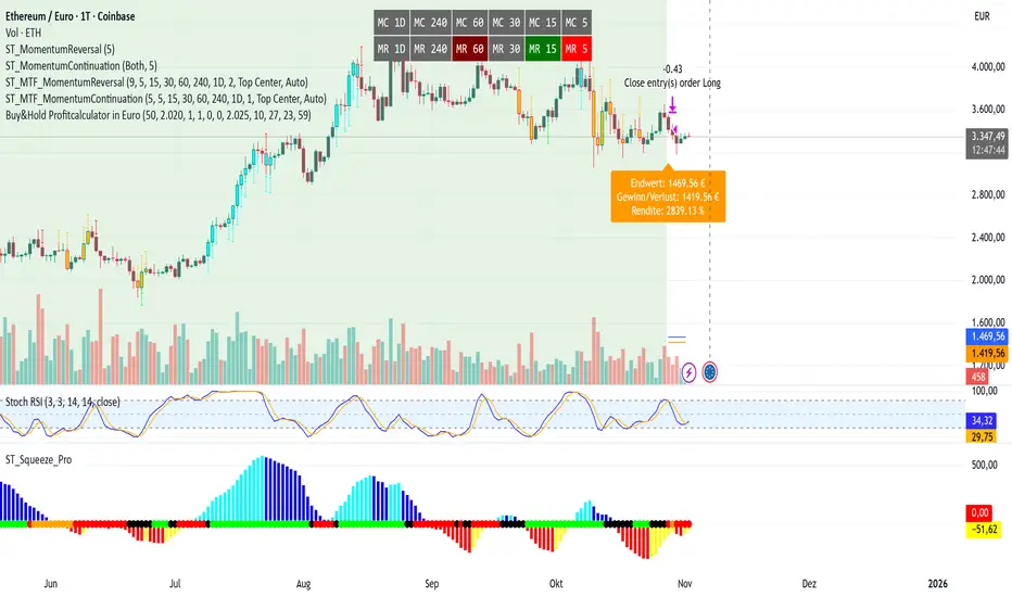
Buy&Hold Profitcalculator in EuroTitle: Buy & Hold Strategy in Euro
Description:
This Pine Script implements a simple yet flexible Buy & Hold strategy denominated in Euros, suitable for a wide range of assets including cryptocurrencies, forex pairs, and stocks.
Key Features:
Custom Investment Amount: Define your invested capital in Euros.
Flexible Start & End Dates: Specify exact entry and exit dates for the strategy.
Automatic Currency Conversion: Supports assets priced in USD or USDT, converting the invested capital to chart currency using the EUR/USD exchange rate.
Single Entry and Exit: Executes a one-time Buy & Hold position based on the defined timeframe.
Profit and Performance Tracking: Calculates total profit/loss in Euros and percentage returns.
Smart Exit Label: Displays a dynamic label at the exit showing final position value, net profit/loss, and return percentage. The label automatically adjusts its position above or below the price bar for optimal visibility.
Visual Enhancements:
Position value and profit/loss plotted on the chart.
Background color highlights the active investment period.
Buy and Sell markers clearly indicate entry and exit points.
This strategy is ideal for traders and investors looking to simulate long-term positions and evaluate performance in Euro terms, even when trading USD-denominated assets.
Usage Notes:
Best used on daily charts for medium- to long-term analysis.
Adjust start and end dates, as well as invested capital, to simulate different scenarios.
Works with any asset, but currency conversion is optimized for USD or USDT-pegged instruments.
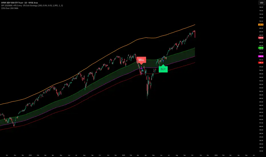
SPY200SMA (+4%/-3%) TQQQ/QQQ STRATEGYSummary of the Improved Strategy: When the price of AMEX:SPY is +4% above the 200SMA BUY NASDAQ:TQQQ and when the price of SPY drops to -3% under the SPY 200SMA SELL everything and slowly DCA into NASDAQ:QQQ over the next 6-12 months or until price returns to +4% above the SPY 200SMA at which point you will go back into 100% TQQQ.
Note: (if the price of QQQ goes 30% above the 200SMA of QQQ deleverage to QQQ or Sell to protect yourself from dot com level event)
More info and stats -https://www.reddit.com/r/LETFs/comments/1nhye66/spy_200sma_43_tqqqqqq_long_term_investment/
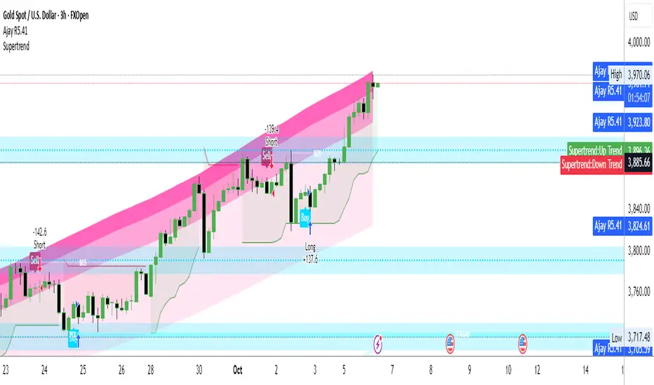
Ajay R5.41🔻 Ajay Gold 3H Power Indicator 🔻
Precision-Based Smart Sell System for Gold (XAU/USD)
💡 Overview
This indicator is specifically designed for Gold (XAU/USD) and delivers best results on the 3-Hour Timeframe (3H TF).
It is a Smart Money Logic-based Sell Confirmation System, combining institutional structure and candle behavior to generate highly accurate bearish signals.
⚙️ Technical Foundation
The indicator uses multiple advanced confirmations:
📉 EMA Trend Filter → Confirms downtrend
💪 RSI Overbought Rejection → Momentum reversal signal
📊 MACD Bearish Cross → Confirms trend strength
🕯️ Bearish Candle Structure → Price action validation
When all conditions align, a clear 🔻 Sell Signal is plotted on the chart.
💎 Hidden Feature
This indicator includes a hidden feature that activates only when the correct market structure forms.
It helps reduce false signals and increases accuracy without being visible on the chart — fully automated internal logic.
📆 Recommended Settings
Symbol: XAU/USD (Gold)
Timeframe: 3-Hour (3H)
Market: Forex / Commodity
Mode: Sell-Only Confirmation Indicator
Performance: Best precision and consistency on 3H TF
📈 How to Use
Select XAU/USD on chart and set 3H timeframe.
Add the indicator to the chart.
Wait for the 🔻 Sell Signal and confirm the market structure after candle close.
Take entry according to your risk management.
⚠️ Disclaimer
This indicator is for educational and analytical purposes only.
No system is 100% accurate — always backtest and demo trade before using in real trading.
💬 Credits
Developed by Ajay Sahu (India)
Based on Institutional & Smart Money Logic
Best results on 3H TF
Hidden Algorithm for XAU/USD traders
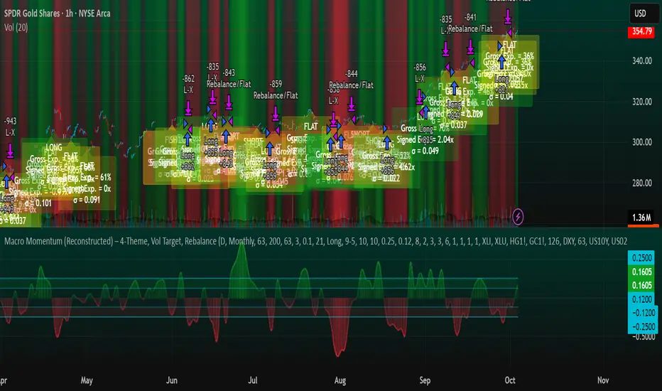
Macro Momentum – 4-Theme, Vol Target, RebalanceMacro Momentum — 4-Theme, Vol Target, Rebalance
Purpose. A macro-aware strategy that blends four economic “themes”—Business Cycle, Trade/USD, Monetary Policy, and Risk Sentiment—into a single, smoothed Composite signal. It then:
gates entries/exits with hysteresis bands,
enforces optional regime filters (200-day bias), and
sizes the position via volatility targeting with caps for long/short exposure.
It’s designed to run on any chart (index, ETF, futures, single stocks) while reading external macro proxies on a chosen Signal Timeframe.
How it works (high level)
Build four theme signals from robust macro proxies:
Business Cycle: XLI/XLU and Copper/Gold momentum, confirmed by the chart’s price vs a long SMA (default 200D).
Trade / USD: DXY momentum (sign-flipped so a rising USD is bearish for risk assets).
Monetary Policy: 10Y–2Y curve slope momentum and 10Y yield trend (steepening & falling 10Y = risk-on; rising 10Y = risk-off).
Risk Sentiment: VIX momentum (bearish if higher) and HYG/IEF momentum (bullish if credit outperforms duration).
Normalize & de-noise.
Optional Winsorization (MAD or stdev) clamps outliers over a lookback window.
Optional Z-score → tanh mapping compresses to ~ for stable weighting.
Theme lines are SMA-smoothed; the final Composite is LSMA-smoothed (linreg).
Decide direction with hysteresis.
Enter/hold long when Composite ≥ Entry Band; enter/hold short when Composite ≤ −Entry Band.
Exit bands are tighter than entry bands to avoid whipsaws.
Apply regime & direction constraints.
Optional Long-only above 200MA (chart symbol) and/or Short-only below 200MA.
Global Direction control (Long / Short / Both) and Invert switch.
Size via volatility targeting.
Realized close-to-close vol is annualized (choose 9-5 or 24/7 market profile).
Target exposure = TargetVol / RealizedVol, capped by Max Long/Max Short multipliers.
Quantity is computed from equity; futures are rounded to whole contracts.
Rebalance cadence & execution.
Trades are placed on Weekly / Monthly / Quarterly rebalance bars or when the sign of exposure flips.
Optional ATR stop/TP for single-stock style risk management.
Inputs you’ll actually tweak
General
Signal Timeframe: Where macro is sampled (e.g., D/W).
Rebalance Frequency: Weekly / Monthly / Quarterly.
ROC & SMA lengths: Defaults for theme momentum and the 200D regime filter.
Normalization: Z-score (tanh) on/off.
Winsorization
Toggle, lookback, multiplier, MAD vs Stdev.
Risk / Sizing
Target Annualized Vol & Realized Vol Lookback.
Direction (Long/Short/Both) and Invert.
Max long/short exposure caps.
Advanced Thresholds
Theme/Composite smoothing lengths.
Entry/Exit bands (hysteresis).
Regime / Execution
Long-only above 200MA, Short-only below 200MA.
Stops/TP (optional)
ATR length and SL/TP multiples.
Theme Weights
Per-theme scalars so you can push/pull emphasis (e.g., overweight Policy during rate cycles).
Macro Proxies
Symbols for each theme (XLI, XLU, HG1!, GC1!, DXY, US10Y, US02Y, VIX, HYG, IEF). Swap to alternatives as needed (e.g., UUP for DXY).
Signals & logic (under the hood)
Business Cycle = ½ ROC(XLI/XLU) + ½ ROC(Copper/Gold), then confirmed by (price > 200SMA ? +1 : −1).
Trade / USD = −ROC(DXY).
Monetary Policy = 0.6·ROC(10Y–2Y) − 0.4·ROC(10Y).
Risk Sentiment = −0.6·ROC(VIX) + 0.4·ROC(HYG/IEF).
Each theme → (optional Winsor) → (robust z or scaled ROC) → tanh → SMA smoothing.
Composite = weighted average → LSMA smoothing → compare to bands → dir ∈ {−1,0,+1}.
Rebalance & flips. Orders fire on your chosen cadence or when the sign of exposure changes.
Position size. exposure = clamp(TargetVol / realizedVol, maxLong/Short) × dir.
Note: The script also exposes Gross Exposure (% equity) and Signed Exposure (× equity) as diagnostics. These can help you audit how vol-targeting and caps translate into sizing over time.
Visuals & alerts
Composite line + columns (color/intensity reflect direction & strength).
Entry/Exit bands with green/red fills for quick polarity reads.
Hidden plots for each Theme if you want to show them.
Optional rebalance labels (direction, gross & signed exposure, σ).
Background heatmap keyed to Composite.
Alerts
Enter/Inc LONG when Composite crosses up (and on rebalance bars).
Enter/Inc SHORT when Composite crosses down (and on rebalance bars).
Exit to FLAT when Composite returns toward neutral (and on rebalance bars).
Practical tips
Start higher timeframes. Daily signals with Monthly rebalance are a good baseline; weekly signals with quarterly rebalances are even cleaner.
Tune Entry/Exit bands before anything else. Wider bands = fewer trades and less noise.
Weights reflect regime. If policy dominates markets, raise Monetary Policy weight; if credit stress drives moves, raise Risk Sentiment.
Proxies are swappable. Use UUP for USD, or futures-continuous symbols that match your data plan.
Futures vs ETFs. Quantity auto-rounds for futures; ETFs accept fractional shares. Check contract multipliers when interpreting exposure.
Caveats
Macro proxies can repaint at the selected signal timeframe as higher-TF bars form; that’s intentional for macro sampling, but test live.
Vol targeting assumes reasonably stationary realized vol over the lookback; if markets regime-shift, revisit volLook and targetVol.
If you disable normalization/winsorization, themes can become spikier; expect more hysteresis band crossings.
What to change first (quick start)
Set Signal Timeframe = D, Rebalance = Monthly, Z-score on, Winsor on (MAD).
Entry/Exit bands: 0.25 / 0.12 (defaults), then nudge until trade count and turnover feel right.
TargetVol: try 10% for diversified indices; lower for single stocks, higher for vol-sell strategies.
Leave weights = 1.0 until you’ve inspected the four theme lines; then tilt deliberately.
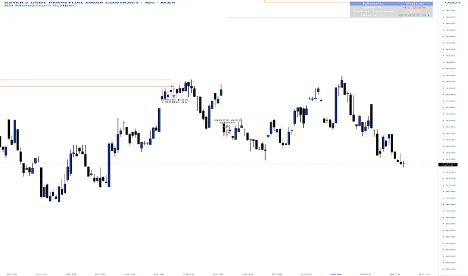
RSI Momentum ScalperOverview
The "RSI Momentum Scalper" is a Pine Script v5 strategy crafted for trading highly volatile markets, with a special focus on newly listed cryptocurrencies. This strategy harnesses the Relative Strength Index (RSI) alongside volume analysis and momentum thresholds to pinpoint short-term trading opportunities. It supports both long and short trades, managed with customizable take profit, stop loss, and trailing stop levels, which are visually plotted on the chart for easy tracking.
Why I Created This Strategy
I developed the "RSI Momentum Scalper" because I was seeking a reliable trading strategy tailored to newly listed, highly volatile cryptocurrencies. These assets often experience rapid price fluctuations, rendering traditional strategies less effective. I aimed to create a tool that could exploit momentum and volume spikes while managing risk through adaptable exit parameters. This strategy is designed to address that need, offering a flexible approach for traders in dynamic crypto markets.
How It Works
The strategy utilizes RSI to identify momentum shifts, combined with volume confirmation, to trigger long or short entries. Trades are controlled with take profit, stop loss, and trailing stop levels, which adjust dynamically as the price moves in your favor. The trailing stop helps lock in profits, while the plotted exit levels provide clear visual cues for trade management.
Customizable Settings
The script is highly customizable, allowing you to adjust it to various market conditions and trading styles. Here’s a brief overview of the key settings:
Trade Mode: Select "Both," "Long Only," or "Short Only" to determine the trade direction.
(Default: Both)
RSI Length: Sets the lookback period for the RSI calculation (2 to 30).
(Default: 8)
A shorter length increases RSI sensitivity, suitable for volatile assets.
RSI Overbought: Defines the upper RSI threshold (60 to 99) for short entries.
(Default: 90)
Higher values signal stronger overbought conditions.
RSI Oversold: Defines the lower RSI threshold (1 to 40) for long entries.
(Default: 10)
Lower values indicate stronger oversold conditions.
RSI Momentum Threshold: Sets the minimum RSI momentum change (1 to 15) to trigger entries.
(Default: 14)
Adjusts the sensitivity to price momentum.
Volume Multiplier: Multiplies the volume moving average to filter high-volume bars (1.0 to 3.0).
(Default: 1)
Higher values require stronger volume confirmation.
Volume MA Length: Sets the lookback period for the volume moving average (5 to 50).
(Default: 13)
Influences the volume trend sensitivity.
Take Profit %: Sets the profit target as a percentage of the entry price (0.1 to 10.0).
(Default: 4.15)
Determines when to close a winning trade.
Stop Loss %: Sets the loss limit as a percentage of the entry price (0.1 to 6.0).
(Default: 1.85)
Protects against significant losses.
Trailing Stop %: Sets the trailing stop distance as a percentage (0.1 to 4.0).
(Default: 2.55)
Locks in profits as the price moves favorably.
Visual Features
Exit Levels: Take profit (green), fixed stop loss (red), and trailing stop (orange) levels are plotted when in a position.
Performance Table: Displays win rate, total trades, and net profit in the top-right corner.
How to Use
Add the strategy to your chart in TradingView.
Adjust the input settings based on the cryptocurrency and timeframe you’re trading.
Monitor the plotted exit levels for trade management.
Use the performance table to assess the strategy’s performance over time.
Notes
Test the strategy on a demo account or with historical data before live trading.
The strategy is optimized for short-term scalping; adjust settings for longer timeframes if needed.
Adaptive MVRV & RSI Strategy V6 (Dynamic Thresholds)Strategy Explanation
This is an advanced Dollar-Cost Averaging (DCA) strategy for Bitcoin that aims to adapt to long-term market cycles and changing volatility. Instead of relying on fixed buy/sell signals, it uses a dynamic, weighted approach based on a combination of on-chain data and classic momentum.
Core Components:
Dual-Indicator Signal: The strategy combines two powerful indicators for a more robust signal:
MVRV Ratio: An on-chain metric to identify when Bitcoin is fundamentally over or undervalued relative to its historical cost basis.
Weekly RSI: A classic momentum indicator to gauge long-term market strength and identify overbought/oversold conditions.
Dynamic, Self-Adjusting Thresholds: The core innovation of this strategy is that it avoids fixed thresholds (e.g., "sell when RSI is 70"). Instead, the buy and sell zones are dynamically calculated based on a long-term (2-year) moving average and standard deviation of each indicator. This allows the strategy to automatically adapt to Bitcoin's decreasing volatility and changing market structure over time.
Weighted DCA (Scaling In & Out): The strategy doesn't just buy or sell a fixed amount. The size of its trades is scaled based on conviction:
Buying: As the MVRV and RSI fall deeper into their "undervalued" zones, the percentage of available cash used for each purchase increases.
Selling: As the indicators rise further into "overvalued" territory, the percentage of the current position sold also increases.
This creates an adaptive system that systematically accumulates during periods of fear and distributes during periods of euphoria, with the intensity of its actions directly tied to the extremity of market conditions.

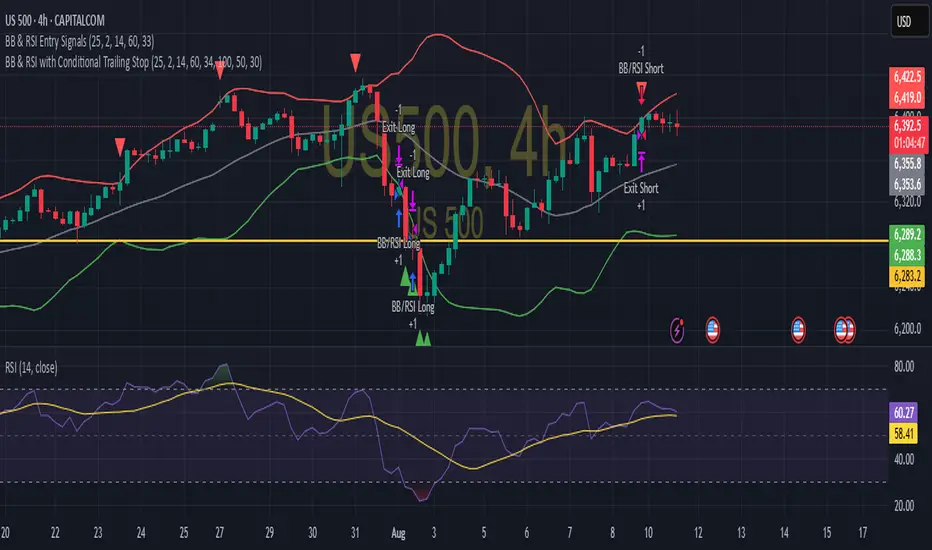
BB & RSI Trailing Stop StrategySimple BB & RSI generated using AI, gets 60% on S&P 500 with the right settings
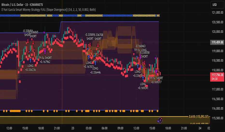
🧪 Yuri Garcia Smart Money Strategy FULL (Slope Divergence))📣 Yuri Garcia – Smart Money Strategy FULL
This is my private Smart Money Concept strategy, designed for my family and community to learn, trade, and grow sustainably.
🔑 How it works:
✅ Volume Cluster Zones: Automatically detects areas where strong buyers or sellers concentrate, acting as dynamic S/R levels.
✅ HTF Institutional Zones (4H): Higher timeframe trend filter ensures you’re always trading in the direction of major flows.
✅ Wick Pullback Filter: Confirms price rejects the zone, catching smart money traps and reversals.
✅ Cumulative Delta (CVD): Confirms whether buyers or sellers are truly in control.
✅ Slope-Based Divergence: Optional hidden divergence between price & CVD to spot reversals others miss.
✅ ATR Dynamic SL/TP: Adapts stop loss and take profit to live volatility with adjustable risk/reward.
🧩 Visual Markers Explained:
🟦 Blue X: Price inside HTF zone
🟨 Yellow X: Price inside Volume Cluster zone
🟧 Orange Circle: Wick pullback detected
🟥 Red Square: CVD confirms order flow strength
🔼 Aqua Triangle Up: Bullish slope divergence
🔽 Purple Triangle Down: Bearish slope divergence
🟢 Green Triangle Up: Final Long Entry confirmed
🔴 Red Triangle Down: Final Short Entry confirmed
⚡ Who is this for?
This strategy is best suited for traders who understand smart money concepts, order flow, and want an adaptive framework to trade major assets like BTC, Gold, SP500, NASDAQ, or FX pairs.
🔒 Important
Use responsibly, backtest extensively, and combine with solid risk management. This is for educational purposes only.
✨ Credits
Built with ❤️ by Yuri Garcia – dedicated to my family & community.
✅ How to use it
1️⃣ Add to chart
2️⃣ Adjust inputs for your asset & timeframe
3️⃣ Enable/disable slope divergence filter to match your style
4️⃣ Set your alerts with built-in conditions
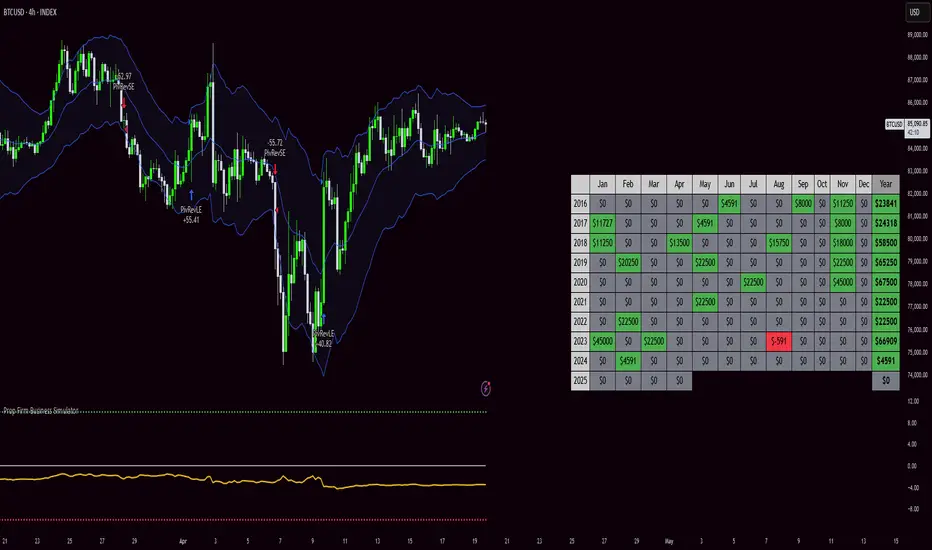
Prop Firm Business SimulatorThe prop firm business simulator is exactly what it sounds like. It's a plug and play tool to test out any tradingview strategy and simulate hypothetical performance on CFD Prop Firms.
Now what is a modern day CFD Prop Firm?
These companies sell simulated trading challenges for a challenge fee. If you complete the challenge you get access to simulated capital and you get a portion of the profits you make on those accounts payed out.
I've included some popular firms in the code as presets so it's easy to simulate them. Take into account that this info will likely be out of date soon as these prices and challenge conditions change.
Also, this tool will never be able to 100% simulate prop firm conditions and all their rules. All I aim to do with this tool is provide estimations.
Now why is this tool helpful?
Most traders on here want to turn their passion into their full-time career, prop firms have lately been the buzz in the trading community and market themselves as a faster way to reach that goal.
While this all sounds great on paper, it is sometimes hard to estimate how much money you will have to burn on challenge fees and set realistic monthly payout expectations for yourself and your trading. This is where this tool comes in.
I've specifically developed this for traders that want to treat prop firms as a business. And as a business you want to know your monthly costs and income depending on the trading strategy and prop firm challenge you are using.
How to use this tool
It's quite simple you remove the top part of the script and replace it with your own strategy. Make sure it's written in same version of pinescript before you do that.
//--$$$$$$$$$$$$$$$$$$$$$$$$$$$$$$$$$$$$$$$$$$$$$$$$--//--------------------------------------------------------------------------------------------------------------------------$$$$$$
//--$$$$$--Strategy-- --$$$$$$--// ******************************************************************************************************************************
//--$$$$$$$$$$$$$$$$$$$$$$$$$$$$$$$$$$$$$$$$$$$$$$$$--//--------------------------------------------------------------------------------------------------------------------------$$$$$$
length = input.int(20, minval=1, group="Keltner Channel Breakout")
mult = input(2.0, "Multiplier", group="Keltner Channel Breakout")
src = input(close, title="Source", group="Keltner Channel Breakout")
exp = input(true, "Use Exponential MA", display = display.data_window, group="Keltner Channel Breakout")
BandsStyle = input.string("Average True Range", options = , title="Bands Style", display = display.data_window, group="Keltner Channel Breakout")
atrlength = input(10, "ATR Length", display = display.data_window, group="Keltner Channel Breakout")
esma(source, length)=>
s = ta.sma(source, length)
e = ta.ema(source, length)
exp ? e : s
ma = esma(src, length)
rangema = BandsStyle == "True Range" ? ta.tr(true) : BandsStyle == "Average True Range" ? ta.atr(atrlength) : ta.rma(high - low, length)
upper = ma + rangema * mult
lower = ma - rangema * mult
//--Graphical Display--// *-*-*-*-*-*-*-*-*-*-*-*-*-*-*-*-*-*-*-*-*-*-*-*-*-*-*-*-*-*-*-*-*-*-*-*-*-*-*-*-*-*-*-*-*-*-*-*-*-*-*-*-*-*-*-*-*-*-*-*-*-*-*-*-*-*-*-*-*-*-*-*-*-$$$$$$
u = plot(upper, color=#2962FF, title="Upper", force_overlay=true)
plot(ma, color=#2962FF, title="Basis", force_overlay=true)
l = plot(lower, color=#2962FF, title="Lower", force_overlay=true)
fill(u, l, color=color.rgb(33, 150, 243, 95), title="Background")
//--Risk Management--// *-*-*-*-*-*-*-*-*-*-*-*-*-*-*-*-*-*-*-*-*-*-*-*-*-*-*-*-*-*-*-*-*-*-*-*-*-*-*-*-*-*-*-*-*-*-*-*-*-*-*-*-*-*-*-*-*-*-*-*-*-*-*-*-*-*-*-*-*-*-*-*-*-*-$$$$$$
riskPerTradePerc = input.float(1, title="Risk per trade (%)", group="Keltner Channel Breakout")
le = high>upper ? false : true
se = lowlower
strategy.entry('PivRevLE', strategy.long, comment = 'PivRevLE', stop = upper, qty=riskToLots)
if se and upper>lower
strategy.entry('PivRevSE', strategy.short, comment = 'PivRevSE', stop = lower, qty=riskToLots)
The tool will then use the strategy equity of your own strategy and use this to simulat prop firms. Since these CFD prop firms work with different phases and payouts the indicator will simulate the gains until target or max drawdown / daily drawdown limit gets reached. If it reaches target it will go to the next phase and keep on doing that until it fails a challenge.
If in one of the phases there is a reward for completing, like a payout, refund, extra it will add this to the gains.
If you fail the challenge by reaching max drawdown or daily drawdown limit it will substract the challenge fee from the gains.
These gains are then visualised in the calendar so you can get an idea of yearly / monthly gains of the backtest. Remember, it is just a backtest so no guarantees of future income.
The bottom pane (non-overlay) is visualising the performance of the backtest during the phases. This way u can check if it is realistic. For instance if it only takes 1 bar on chart to reach target you are probably risking more than the firm wants you to risk. Also, it becomes much less clear if daily drawdown got hit in those high risk strategies, the results will be less accurate.
The daily drawdown limit get's reset every time there is a new dayofweek on chart.
If you set your prop firm preset setting to "'custom" the settings below that are applied as your prop firm settings. Otherwise it will use one of the template by default it's FTMO 100K.
The strategy I'm using as an example in this script is a simple Keltner Channel breakout strategy. I'm using a 0.05% commission per trade as that is what I found most common on crypto exchanges and it's close to the commissions+spread you get on a cfd prop firm. I'm targeting a 1% risk per trade in the backtest to try and stay within prop firm boundaries of max 1% risk per trade.
Lastly, the original yearly and monthly performance table was developed by Quantnomad and I've build ontop of that code. Here's a link to the original publication:
That's everything for now, hope this indicator helps people visualise the potential of prop firms better or to understand that they are not a good fit for their current financial situation.
50 EMA Crossover With Monthly DCARecommended Chart Interval = 1W
Overview:
This strategy combines trend-following principles with dollar-cost averaging (DCA), aiming to efficiently deploy capital while minimizing market timing risk.
How It Works:
When the Long Condition is Not Met (i.e., Price < 50 EMA):
- If the price is below the 50 EMA, a fixed DCA amount is added to a cash reserve every month.
- This ensures that capital is consistently accumulated, even when the strategy isn't in a long position.
When the Long Condition is Met (i.e., Price > 50 EMA):
- A long position is opened when the price is above the 50 EMA.
- At this point, the entire capital, including the accumulated cash reserve, is deployed into the market.
- While the strategy is long, a DCA buy order is placed every month using the set DCA amount, continuously investing as the market conditions allow.
Exit Strategy:
If the price falls below the 50 EMA, the strategy closes all positions, and the cash reserve accumulation process begins again.
Key Benefits:
✔ Systematic Investing: Ensures consistent capital deployment while following trend signals.
✔ Cash Efficiency: Accumulates uninvested funds when conditions aren’t met and deploys them at optimal moments.
✔ Risk Management: Exits when the price trend weakens, protecting capital.
Conclusion:
This method allows for efficient capital growth by combining a trend-following approach with disciplined DCA, ensuring risk is managed while capital is deployed systematically at optimal points in the market. 🚀
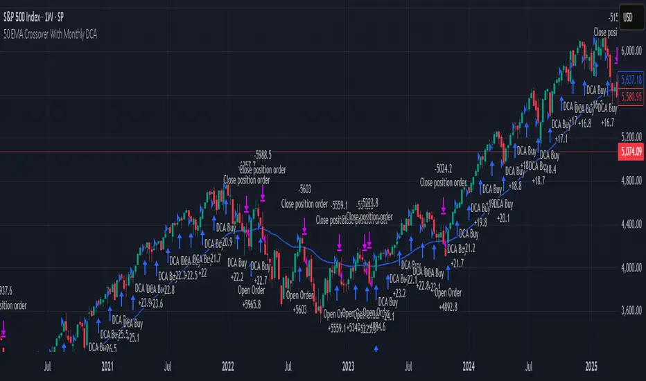
Z-Score Normalized VIX StrategyThis strategy leverages the concept of the Z-score applied to multiple VIX-based volatility indices, specifically designed to capture market reversals based on the normalization of volatility. The strategy takes advantage of VIX-related indicators to measure extreme levels of market fear or greed and adjusts its position accordingly.
1. Overview of the Z-Score Methodology
The Z-score is a statistical measure that describes the position of a value relative to the mean of a distribution in terms of standard deviations. In this strategy, the Z-score is calculated for various volatility indices to assess how far their values are from their historical averages, thus normalizing volatility levels. The Z-score is calculated as follows:
Z = \frac{X - \mu}{\sigma}
Where:
• X is the current value of the volatility index.
• \mu is the mean of the index over a specified period.
• \sigma is the standard deviation of the index over the same period.
This measure tells us how many standard deviations the current value of the index is away from its average, indicating whether the market is experiencing unusually high or low volatility (fear or calm).
2. VIX Indices Used in the Strategy
The strategy utilizes four commonly referenced volatility indices:
• VIX (CBOE Volatility Index): Measures the market’s expectations of 30-day volatility based on S&P 500 options.
• VIX3M (3-Month VIX): Reflects expectations of volatility over the next three months.
• VIX9D (9-Day VIX): Reflects shorter-term volatility expectations.
• VVIX (VIX of VIX): Measures the volatility of the VIX itself, indicating the level of uncertainty in the volatility index.
These indices provide a comprehensive view of the current volatility landscape across different time horizons.
3. Strategy Logic
The strategy follows a long entry condition and an exit condition based on the combined Z-score of the selected volatility indices:
• Long Entry Condition: The strategy enters a long position when the combined Z-score of the selected VIX indices falls below a user-defined threshold, indicating an abnormally low level of volatility (suggesting a potential market bottom and a bullish reversal). The threshold is set as a negative value (e.g., -1), where a more negative Z-score implies greater deviation below the mean.
• Exit Condition: The strategy exits the long position when the combined Z-score exceeds the threshold (i.e., when the market volatility increases above the threshold, indicating a shift in market sentiment and reduced likelihood of continued upward momentum).
4. User Inputs
• Z-Score Lookback Period: The user can adjust the lookback period for calculating the Z-score (e.g., 6 periods).
• Z-Score Threshold: A customizable threshold value to define when the market has reached an extreme volatility level, triggering entries and exits.
The strategy also allows users to select which VIX indices to use, with checkboxes to enable or disable each index in the calculation of the combined Z-score.
5. Trade Execution Parameters
• Initial Capital: The strategy assumes an initial capital of $20,000.
• Pyramiding: The strategy does not allow pyramiding (multiple positions in the same direction).
• Commission and Slippage: The commission is set at $0.05 per contract, and slippage is set at 1 tick.
6. Statistical Basis of the Z-Score Approach
The Z-score methodology is a standard technique in statistics and finance, commonly used in risk management and for identifying outliers or unusual events. According to Dumas, Fleming, and Whaley (1998), volatility indices like the VIX serve as a useful proxy for market sentiment, particularly during periods of high uncertainty. By calculating the Z-score, we normalize volatility and quantify the degree to which the current volatility deviates from historical norms, allowing for systematic entry and exit based on these deviations.
7. Implications of the Strategy
This strategy aims to exploit market conditions where volatility has deviated significantly from its historical mean. When the Z-score falls below the threshold, it suggests that the market has become excessively calm, potentially indicating an overreaction to past market events. Entering long positions under such conditions could capture market reversals as fear subsides and volatility normalizes. Conversely, when the Z-score rises above the threshold, it signals increased volatility, which could be indicative of a bearish shift in the market, prompting an exit from the position.
By applying this Z-score normalized approach, the strategy seeks to achieve more consistent entry and exit points by reducing reliance on subjective interpretation of market conditions.
8. Scientific Sources
• Dumas, B., Fleming, J., & Whaley, R. (1998). “Implied Volatility Functions: Empirical Tests”. The Journal of Finance, 53(6), 2059-2106. This paper discusses the use of volatility indices and their empirical behavior, providing context for volatility-based strategies.
• Black, F., & Scholes, M. (1973). “The Pricing of Options and Corporate Liabilities”. Journal of Political Economy, 81(3), 637-654. The original Black-Scholes model, which forms the basis for many volatility-related strategies.
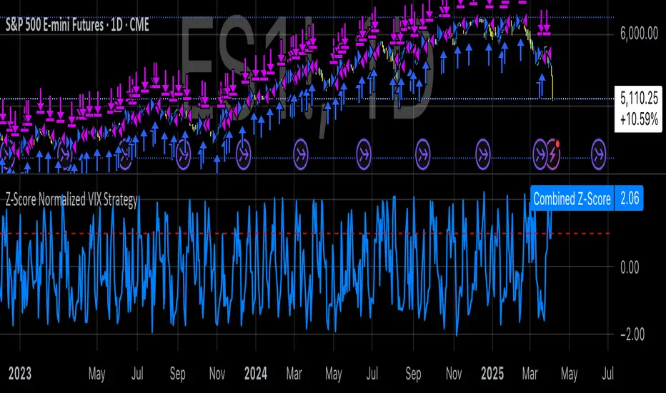
EMA Crossover (Short Focus with Trailing Stop)This strategy utilizes a combination of Exponential Moving Averages (EMA) and Simple Moving Averages (SMA) to generate entry and exit signals for both long and short positions. The core of the strategy is based on the 13-period EMA (short EMA) crossing the 33-period EMA (long EMA) for entering long trades, while a 13-period EMA crossing the 25-period EMA (mid EMA) generates short trade signals. The 100-period SMA and 200-period SMA serve as additional trend indicators to provide context for the market conditions. The strategy aims to capitalize on trend reversals and momentum shifts in the market.
The strategy is designed to execute trades swiftly with an emphasis on entering positions when conditions align in real time. For long entries, the strategy initiates a buy when the 13 EMA is greater than the 33 EMA, indicating a bullish trend. For short entries, the 13 EMA crossing below the 33 EMA signals a bearish trend, prompting a short position. Importantly, the code includes built-in exit conditions for both long and short positions. Long positions are exited when the 13 EMA falls below the 33 EMA, while short positions are closed when the 13 EMA crosses above the 25 EMA.
A key feature of the strategy is the use of trailing stops for both long and short positions. This dynamic exit method adjusts the stop level as the market moves in favor of the trade, locking in profits while reducing the risk of losses. The trailing stop for long positions is based on the high price of the current bar, while the trailing stop for short positions is set using the low price, providing more flexibility in managing risk. This trailing stop mechanism helps to capture profits from favorable market moves while ensuring that positions are exited if the market moves against them.
This strategy works best on the daily timeframe and is optimized for major cryptocurrency pairs. The daily chart allows for the EMAs to provide more reliable signals, as the strategy is designed to capture broader trends rather than short-term market fluctuations. Using it on major crypto pairs increases its effectiveness as these assets tend to have strong and sustained trends, providing better opportunities for the strategy to perform well.
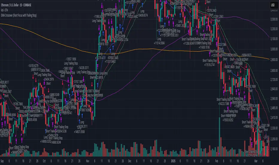
JMA Quantum Edge: Adaptive Precision Trading System JMA Quantum Edge: Adaptive Precision Trading System - Enhanced Visuals & Risk Management
Get ready to experience a groundbreaking trading strategy that adapts in real-time to market conditions! This powerful, open-source script combines advanced technical analysis with state-of-the-art risk management tools, designed to give you the edge you need in today's dynamic markets.
What It Does:
Adaptive JMA Indicator:
Utilizes a custom Jurik Moving Average (JMA) that adjusts its sensitivity based on market volatility, ensuring you get precise signals even in the most fluctuating environments.
Dynamic Risk Management:
Features built-in support for partial exits (scaling out) to secure profits, along with an optional Kelly Criterion-based position sizing that tailors your exposure based on historical performance metrics.
Robust Error Handling:
Incorporates market condition filters—like minimum volume and maximum allowed gap percentage—to ensure trades are only executed under favorable conditions.
Vivid Visual Enhancements:
Enjoy an animated background that reflects market momentum, dynamic pivot markers, and clearly drawn trend channels. Plus, interactive tables provide real-time performance analytics and detailed error metrics.
Fully Customizable:
With a comprehensive set of inputs, you can easily tailor the strategy to your personal trading style and market preferences. Adjust everything from JMA parameters to refresh intervals for tables and labels!
How to Use It:
Add the Script:
Copy and paste the script into the Pine Script Editor on TradingView and click “Add to Chart.”
Configure Your Settings:
Customize your risk management (capital, commission, position sizing, partial exits, etc.) and tweak the JMA settings to match your preferred trading style. Use the extensive input panel to adjust visuals, alerts, and more.
Backtest & Optimize:
Run the strategy in the Strategy Tester to analyze its historical performance. Monitor real-time analytics and error metrics via the interactive tables, and fine-tune your parameters for optimal performance.
Go Live with Confidence:
Once you're satisfied with the backtest results, use the generated signals for live trading, and let the system help you stay ahead in fast-paced markets!
How to use the imputs:
This cutting-edge strategy is designed to adapt to changing market conditions and offers you complete control over your trading parameters. Here’s a breakdown of what each group of inputs does and how you should use them:
Risk Management & Trade Settings
Recalculate on Every Tick:
What it does: When enabled, the strategy recalculates on every price update.
Recommendation: Leave it true for fast charts.
Initial Capital:
What it does: Sets your starting capital for backtesting, which influences position sizing and performance metrics.
Recommendation: Start with $10,000 (or adjust according to your trading capital).
Commission (%):
What it does: Simulates the cost per trade.
Recommendation: Use a realistic rate (e.g., 0.04%).
Position Size & Quantity Type:
What they do: Define how large each trade will be. Choose between a fixed unit amount or a percentage of equity.
Recommendation: For beginners, the default fixed value is a good start. Experiment later with percentage-based sizing if needed.
Order Comment:
What it does: Adds a label to your orders for easier tracking.
Allow Reverse Orders:
What it does: If disabled, the strategy will close opposing positions before entering a new trade, reducing conflicts.
Enable Dynamic Position Sizing:
What it does: Adjusts trade size based on current volatility.
Recommendation: Beginners may start with this disabled until they understand basic sizing.
Partial Exit Inputs:
What they do:
Enable Partial Exits: When turned on, you can scale out of your position to lock in profits.
Partial Exit Profit (%): The profit percentage that triggers a partial exit.
Partial Exit Percentage: The percentage of your current position to exit. Recommendation: Use defaults (e.g., 5% profit, 50% exit) to secure profits gradually.
Kelly Criterion Option:
What it does: When enabled, adjusts your position sizing using historical performance (win rate and profit factor).
Recommendation: Beginners might leave this disabled until comfortable with backtest performance metrics.
Market Condition Filters:
What they do:
Minimum Volume: Ensures trades occur only when there’s sufficient market activity.
Maximum Gap (%): Prevents trading if there’s an unusually large gap between the previous close and current open. Recommendation: Defaults work well for most markets. If trades seem erratic, consider tightening these limits.
JMA Settings
Price Source:
What it does: The input series for the JMA calculation, typically set to the closing price.
JMA Length:
What it does: Controls the smoothing period of the JMA. Lower values are more sensitive; higher values smooth out the noise. Recommendation: Start with 21.
JMA Phase & Power:
What they do: Adjust how responsive the JMA is. Phase controls timing; power adjusts the intensity. Recommendation: Default settings (63 phase and 3 power) are a balanced starting point.
Visual Settings & Style
Show JMA Line, Pivot Lines, and Pivot Labels:
What they do: Toggle visual elements on your chart for easier signal identification.
Pivot History Count:
What it does: Limits how many historical pivot markers are displayed.
Color Settings (Up/Down Neon Colors):
What they do: Set the visual cues for buy and sell signals.
Pivot Marker & Line Style:
What they do: Choose the style and thickness of your pivot markers and lines.
Show Stats Panel:
What it does: Displays real-time performance and error metrics.
Dynamic Background & Visual Enhancements
Animate Background:
What it does: Changes the background color based on market momentum.
Show Trend Channels & Volume Zones:
What they do: Draw trend channels and highlight areas of high volatility/volume.
Show Data-Rich Labels:
What it does: Displays key metrics like volume, error percentage, and momentum on the chart.
High Volatility Threshold:
What it does: Determines the multiplier for when the chart background should change due to high volatility.
Multi-Timeframe Settings
Higher Timeframe:
What it does: Uses a higher timeframe’s JMA for trend confirmation. Recommendation: Use Daily ('D') or Weekly ('W') for broader trend analysis.
Show HTF Trend Zone & Opacity:
What they do: Display a visual zone from the higher timeframe to help confirm trends.
6. Trailing Stop Settings
Trailing Stop ATR Factor & Offset Multiplier:
What they do: Calculate trailing stops based on the Average True Range (ATR), adjusting stop distances dynamically. Recommendation: Default settings are a good balance but can be fine-tuned based on asset volatility.
Alerts & Notifications
Alerts on Pivot Formation & JMA Crossover:
What they do: Notify you when key events occur.
Dynamic Power Threshold:
What it does: Sets the sensitivity for dynamic alerts.
8. Static Stop Loss / Take Profit
Static Stop Loss (%) & Take Profit (%):
What they do: Allow you to set fixed stop loss or take profit levels. Recommendation: Leave them at 0 to disable if you prefer dynamic risk management, or set them if you have strict risk/reward preferences.
Advanced Settings
ATR Length:
What it does: Determines the period for ATR calculation, impacting trailing stop sensitivity. Recommendation: Start with 14.
Optimization Feedback & Enhanced Error Analysis
Error Metric Length & Error Threshold (%):
What they do: Calculate error metrics (like average error, skewness, and kurtosis) to help you fine-tune the JMA. Recommendation: Use the defaults and adjust if the error metrics seem off during backtesting.
UI - User-Driven Tweaking & Table Customization
Parameter Tweaker Panel, Debug/Performance Table Settings:
What they do: Provide interactive tables that display real-time performance, error metrics, and allow you to monitor strategy parameters.
Refresh Frequency Options (Table & Label Refresh Intervals):
What they do: Set how often the tables and labels update.
Recommendation: Start with an interval of 1 bar; increase it if your chart is too busy.
Important for Beginners:
Default Settings:
All default values have been chosen for balanced performance across different markets. If you ever experience unexpected behavior, start by resetting the inputs to their defaults.
Step-by-Step Adjustments:
Experiment by changing one setting at a time while observing how the strategy’s signals and performance metrics change. This will help you understand the impact of each parameter.
Resetting to Defaults:
If things seem off or you’re not getting the expected results, you can always reset the indicator. Either reload the script or use the “Reset Inputs” option (if available) to revert to the default settings.
Jump in, experiment, and enjoy the power of adaptive precision trading. This strategy is built to grow with your skills—have fun exploring and refining your trading edge!
Happy trading!

Gold Pro StrategyHere’s the strategy description in a chat format:
---
**Gold (XAU/USD) Trend-Following Strategy**
This **trend-following strategy** is designed for trading gold (XAU/USD) by combining moving averages, MACD momentum indicators, and RSI filters to capture sustained trends while managing volatility risks. The strategy uses volatility-adjusted stops to protect gains and prevent overexposure during erratic price movements. The aim is to take advantage of trending markets by confirming momentum and ensuring entries are not made at extreme levels.
---
**Key Components**
1. **Trend Identification**
- **50 vs 200 EMA Crossover**
- **Bullish Trend:** 50 EMA crosses above 200 EMA, and the price closes above the 200 EMA
- **Bearish Trend:** 50 EMA crosses below 200 EMA, and the price closes below the 200 EMA
2. **Momentum Confirmation**
- **MACD (12,26,9)**
- **Buy Signal:** MACD line crosses above the signal line
- **Sell Signal:** MACD line crosses below the signal line
- **RSI (14 Period)**
- **Bullish Zone:** RSI between 50-70 to avoid overbought conditions
- **Bearish Zone:** RSI between 30-50 to avoid oversold conditions
3. **Entry Criteria**
- **Long Entry:** Bullish trend, MACD bullish crossover, and RSI between 50-70
- **Short Entry:** Bearish trend, MACD bearish crossover, and RSI between 30-50
4. **Exit & Risk Management**
- **ATR Trailing Stops (14 Period):**
- Initial Stop: 3x ATR from entry price
- Trailing Stop: Adjusts to lock in profits as price moves favorably
- **Position Sizing:** 100% of equity per trade (high-risk strategy)
---
**Key Logic Flow**
1. **Trend Filter:** Use the 50/200 EMA relationship to define the market's direction
2. **Momentum Confirmation:** Confirm trend momentum with MACD crossovers
3. **RSI Validation:** Ensure RSI is within non-extreme ranges before entering trades
4. **Volatility-Based Risk Management:** Use ATR stops to manage market volatility
---
**Visual Cues**
- **Blue Line:** 50 EMA
- **Red Line:** 200 EMA
- **Green Triangles:** Long entry signals
- **Red Triangles:** Short entry signals
---
**Strengths**
- **Clear Trend Focus:** Avoids counter-trend trades
- **RSI Filter:** Prevents entering overbought or oversold conditions
- **ATR Stops:** Adapts to gold’s inherent volatility
- **Simple Rules:** Easy to follow with minimal inputs
---
**Weaknesses & Risks**
- **Infrequent Signals:** 50/200 EMA crossovers are rare
- **Potential Missed Opportunities:** Strict RSI criteria may miss some valid trends
- **Aggressive Position Sizing:** 100% equity allocation can lead to large drawdowns
- **No Profit Targets:** Relies on trailing stops rather than defined exit targets
---
**Performance Profile**
| Metric | Expected Range |
|----------------------|---------------------|
| Annual Trades | 4-8 |
| Win Rate | 55-65% |
| Max Drawdown | 25-35% |
| Profit Factor | 1.8-2.5 |
---
**Optimization Recommendations**
1. **Increase Trade Frequency**
Adjust the EMAs to shorter periods:
- `emaFastLen = input.int(30, "Fast EMA")`
- `emaSlowLen = input.int(150, "Slow EMA")`
2. **Relax RSI Filters**
Adjust the RSI range to:
- `rsiBullish = rsi > 45 and rsi < 75`
- `rsiBearish = rsi < 55 and rsi > 25`
3. **Add Profit Targets**
Introduce a profit target at 1.5% above entry:
```pine
strategy.exit("Long Exit", "Long",
stop=longStopPrice,
profit=close*1.015, // 1.5% target
trail_offset=trailOffset)
```
4. **Reduce Position Sizing**
Risk a smaller percentage per trade:
- `default_qty_value=25`
---
**Best Use Case**
This strategy excels in **strong trending markets** such as gold rallies during economic or geopolitical crises. However, during sideways or choppy market conditions, the strategy might require manual intervention to avoid false signals. Additionally, integrating fundamental analysis—like monitoring USD weakness or geopolitical risks—can enhance its effectiveness.
---
This strategy offers a balanced approach for trading gold, combining trend-following principles with risk management tailored to the volatility of the market.

Bollinger Bands Mean Reversion by Kevin Davey Bollinger Bands Mean Reversion Strategy Description
The Bollinger Bands Mean Reversion Strategy is a popular trading approach based on the concept of volatility and market overreaction. The strategy leverages Bollinger Bands, which consist of an upper and lower band plotted around a central moving average, typically using standard deviations to measure volatility. When the price moves beyond these bands, it signals potential overbought or oversold conditions, and the strategy seeks to exploit a reversion back to the mean (the central band).
Strategy Components:
1. Bollinger Bands:
The bands are calculated using a 20-period Simple Moving Average (SMA) and a multiple (usually 2.0) of the standard deviation of the asset’s price over the same period. The upper band represents the SMA plus two standard deviations, while the lower band is the SMA minus two standard deviations. The distance between the bands increases with higher volatility and decreases with lower volatility.
2. Mean Reversion:
Mean reversion theory suggests that, over time, prices tend to move back toward their historical average. In this strategy, a buy signal is triggered when the price falls below the lower Bollinger Band, indicating a potential oversold condition. Conversely, the position is closed when the price rises back above the upper Bollinger Band, signaling an overbought condition.
Entry and Exit Logic:
Buy Condition: The strategy enters a long position when the price closes below the lower Bollinger Band, anticipating a mean reversion to the central band (SMA).
Sell Condition: The long position is exited when the price closes above the upper Bollinger Band, implying that the market is likely overbought and a reversal could occur.
This approach uses mean reversion principles, aiming to capitalize on short-term price extremes and volatility compression, often seen in sideways or non-trending markets. Scientific studies have shown that mean reversion strategies, particularly those based on volatility indicators like Bollinger Bands, can be effective in capturing small but frequent price reversals  .
Scientific Basis for Bollinger Bands:
Bollinger Bands, developed by John Bollinger, are widely regarded in both academic literature and practical trading as an essential tool for volatility analysis and mean reversion strategies. Research has shown that Bollinger Bands effectively identify relative price highs and lows, and can be used to forecast price volatility and detect potential breakouts . Studies in financial markets, such as those by Fernández-Rodríguez et al. (2003), highlight the efficacy of Bollinger Bands in detecting overbought or oversold conditions in various assets .
Who is Kevin Davey?
Kevin Davey is an award-winning algorithmic trader and highly regarded expert in developing and optimizing systematic trading strategies. With over 25 years of experience, Davey gained significant recognition after winning the prestigious World Cup Trading Championships multiple times, where he achieved triple-digit returns with minimal drawdown. His success has made him a key figure in algorithmic trading education, with a focus on disciplined and rule-based trading systems.

Williams %R StrategyThe Williams %R Strategy implemented in Pine Script™ is a trading system based on the Williams %R momentum oscillator. The Williams %R indicator, developed by Larry Williams in 1973, is designed to identify overbought and oversold conditions in a market, helping traders time their entries and exits effectively (Williams, 1979). This particular strategy aims to capitalize on short-term price reversals in the S&P 500 (SPY) by identifying extreme values in the Williams %R indicator and using them as trading signals.
Strategy Rules:
Entry Signal:
A long position is entered when the Williams %R value falls below -90, indicating an oversold condition. This threshold suggests that the market may be near a short-term bottom, and prices are likely to reverse or rebound in the short term (Murphy, 1999).
Exit Signal:
The long position is exited when:
The current close price is higher than the previous day’s high, or
The Williams %R indicator rises above -30, indicating that the market is no longer oversold and may be approaching an overbought condition (Wilder, 1978).
Technical Analysis and Rationale:
The Williams %R is a momentum oscillator that measures the level of the close relative to the high-low range over a specific period, providing insight into whether an asset is trading near its highs or lows. The indicator values range from -100 (most oversold) to 0 (most overbought). When the value falls below -90, it indicates an oversold condition where a reversal is likely (Achelis, 2000). This strategy uses this oversold threshold as a signal to initiate long positions, betting on mean reversion—an established principle in financial markets where prices tend to revert to their historical averages (Jegadeesh & Titman, 1993).
Optimization and Performance:
The strategy allows for an adjustable lookback period (between 2 and 25 days) to determine the range used in the Williams %R calculation. Empirical tests show that shorter lookback periods (e.g., 2 days) yield the most favorable outcomes, with profit factors exceeding 2. This finding aligns with studies suggesting that shorter timeframes can effectively capture short-term momentum reversals (Fama, 1970; Jegadeesh & Titman, 1993).
Scientific Context:
Mean Reversion Theory: The strategy’s core relies on mean reversion, which suggests that prices fluctuate around a mean or average value. Research shows that such strategies, particularly those using oscillators like Williams %R, can exploit these temporary deviations (Poterba & Summers, 1988).
Behavioral Finance: The overbought and oversold conditions identified by Williams %R align with psychological factors influencing trading behavior, such as herding and panic selling, which often create opportunities for price reversals (Shiller, 2003).
Conclusion:
This Williams %R-based strategy utilizes a well-established momentum oscillator to time entries and exits in the S&P 500. By targeting extreme oversold conditions and exiting when these conditions revert or exceed historical ranges, the strategy aims to capture short-term gains. Scientific evidence supports the effectiveness of short-term mean reversion strategies, particularly when using indicators sensitive to momentum shifts.
References:
Achelis, S. B. (2000). Technical Analysis from A to Z. McGraw Hill.
Fama, E. F. (1970). Efficient Capital Markets: A Review of Theory and Empirical Work. The Journal of Finance, 25(2), 383-417.
Jegadeesh, N., & Titman, S. (1993). Returns to Buying Winners and Selling Losers: Implications for Stock Market Efficiency. The Journal of Finance, 48(1), 65-91.
Murphy, J. J. (1999). Technical Analysis of the Financial Markets: A Comprehensive Guide to Trading Methods and Applications. New York Institute of Finance.
Poterba, J. M., & Summers, L. H. (1988). Mean Reversion in Stock Prices: Evidence and Implications. Journal of Financial Economics, 22(1), 27-59.
Shiller, R. J. (2003). From Efficient Markets Theory to Behavioral Finance. Journal of Economic Perspectives, 17(1), 83-104.
Williams, L. (1979). How I Made One Million Dollars… Last Year… Trading Commodities. Windsor Books.
Wilder, J. W. (1978). New Concepts in Technical Trading Systems. Trend Research.
This explanation provides a scientific and evidence-based perspective on the Williams %R trading strategy, aligning it with fundamental principles in technical analysis and behavioral finance.
